INDEX Match to show a tie

[charismaman]

Hi,

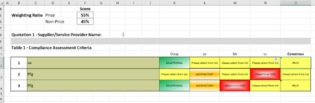
I am seeking help in a formula to show the results from evaluation that either shows if the consensus is either Exceptional, Satisfactory, Unsatisfactory or if it the outcome is a tied result based on the evaluation selection from other cells.

Column "O" should show the consensus of "K-N" but I cant seem to figure it out.

I have attached a sample with drop list selection for "K-N"

Thanks in advance

 

[ExceLoki]

let me know if this works for you
---------------------

Book1
	A	B	C	D	E	F	G	H	I
11					Doug	aa	bb	cc	Consensus
12	Validation		1	aa	Exceptional	Please Select from list	Please Select from list	Please Select from list	Please Select from list
13	Please Select from list		2	fffg	Please Select from list	Satisfactory	Please Select from list	Unsatisfactory	Please Select from list
14	Exceptional		3	fffg	Exceptional	Satisfactory	Unsatisfactory	Please Select from list	Tied Result
15	Satisfactory
16	Unsatisfactory
Sheet1

Cell Formulas
Range	Formula
I12:I14	I12	=IFERROR(INDEX(E12:H12,MODE(MATCH(E12:H12,E12:H12,0))),"Tied Result")

Cells with Data Validation
Cell	Allow	Criteria
E12:H14	List	=$A$13:$A$16

 

[charismaman]

Hi Thanks,

It works on some of the cells, sometimes it doesnt show a tie.

 

[charismaman]

Sorry I forgot to mention that the selection of exceptional, Satisfactory, Unsatisfactory is from a drop down list

 

[ExceLoki]

if you are able to put some helper rows, i think i've come up with a solution. try this and let me know if it works for you
-----------------------

Book1
	A	B	C	D	E	F	G	H	I	J	K	L	M	N
1			Doug	Bob	Ralp	Chris		Please Select from list	Validation	Exceptional	Satisfactory	Unsatisfactory		Consensus
2	1	aa	Exceptional	Please Select from list	Please Select from list	Please Select from list		3	0	1	0	0		Please Select from list
3	2	fffg	Please Select from list	Satisfactory	Please Select from list	Unsatisfactory		2	0	0	1	1		Please Select from list
4	3	fffg	Exceptional	Satisfactory	Unsatisfactory	Please Select from list		1	0	1	1	1		Tied Result
5	4	123	Unsatisfactory	Satisfactory	Satisfactory	Unsatisfactory		0	0	0	2	2		Tied Result
6	5	456	Unsatisfactory	Please Select from list	Please Select from list	Unsatisfactory		2	0	0	0	2		Tied Result
7	6	789	Exceptional	Unsatisfactory	Satisfactory	Please Select from list		1	0	1	1	1		Tied Result
8	7	987	Exceptional	Exceptional	Exceptional	Please Select from list		1	0	3	0	0		Exceptional
9	8	654	Satisfactory	Satisfactory	Unsatisfactory	Exceptional		0	0	1	2	1		Satisfactory
10	9	321	Exceptional	Exceptional	Exceptional	Please Select from list		1	0	3	0	0		Exceptional
Sheet2

Cell Formulas
Range	Formula
H2:L10	H2	=COUNTIF($C2:$F2,H$1)
N2:N10	N2	=IF(LARGE(H2:L2,1)=LARGE(H2:L2,2),"Tied Result",XLOOKUP(LARGE(H2:L2,1),H2:L2,$H$1:$L$1))

Cells with Data Validation
Cell	Allow	Criteria
C2:F10	List	=$H$1:$L$1