Hi folks,
I am not very versant with chart objects and keep getting stuck with the following problem. Thanks for your help!
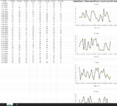
I have put a simple version of a minisheet below with data. I could not figure out how to capture the charts in the minisheet so an image of the "desired result" is also uploaded.
What I am trying to do.
What I was thinking...but does not work
I am not very versant with chart objects and keep getting stuck with the following problem. Thanks for your help!
I have put a simple version of a minisheet below with data. I could not figure out how to capture the charts in the minisheet so an image of the "desired result" is also uploaded.
What I am trying to do.
- I want to automatically create scatter charts for every second row of data where the the X data is always the A1 (Date) column, but the Y data is every nth+2 column (Tons).
- Add chart title that equals the header value for that column
- Put the chart below the previous chart offset by some increment to the top so they are evenly spaced
- Make the chart object name equal also to the header name so that by the end of the loop each chart object has its own name so I can reference them elsewhere.
What I was thinking...but does not work
VBA Code:
Sub ChartMaker()

Dim rng As Range
Dim rowNum As Long
Dim topInc As Long


Sheets("Charts").Activate

rowNum = 2
topInc = 300

For Each rng In Range("B2:I2").Columns

    Dim chartObj As ChartObject
    Dim refChart As Chart

    Set chartObj = ActiveSheet.ChartObjects.Add(Top:=10 + topInc, Left:=325, Width:=600, Height:=300) 'place the next chart incrementally below the previous chart until all charts are made..
    Set refChart = chartObj.Chart
    refChart.ChartType = xlXYScatter
    refChart.SetSourceData Source:=Range(Cells(2, rowNum), Cells(30, 2)) 'Getting lost here, I dont quite know how to set X (date) and Y data separately

    ActiveChart.SetElement (msoElementChartTitleAboveChart)
        ActiveChart.ChartTitle.Text = Cell(2, rowNum) 'Trying to add chart title equal to the header like A Tons or B Tons

    With Chart
        .Parent.Name = rowNum 'would like chart object name to be equal to the header like A_Tons or B_Tons, etc

    End If

rowNum = rowNum + 2 'idea is to make a chart for every second row.

Next rng

End Sub| Book2.xlsx | |||||||||||
|---|---|---|---|---|---|---|---|---|---|---|---|
| A | B | C | D | E | F | G | H | I | |||
| 1 | Date | A Tons | A Over | B Tons | B Over | C Tons | C Over | D Tons | D Over | ||
| 2 | 6/3/2022 | 13 | 1 | 59 | 47 | 27 | 15 | 38 | 26 | ||
| 3 | 6/2/2022 | 13 | 1 | 14 | 2 | 15 | 3 | 42 | 30 | ||
| 4 | 6/1/2022 | 42 | 30 | 17 | 5 | 29 | 17 | 26 | 14 | ||
| 5 | 5/31/2022 | 63 | 51 | 33 | 21 | 41 | 29 | 67 | 55 | ||
| 6 | 5/30/2022 | 50 | 38 | 52 | 40 | 23 | 11 | 13 | 1 | ||
| 7 | 5/29/2022 | 41 | 29 | 46 | 34 | 38 | 26 | 74 | 62 | ||
| 8 | 5/28/2022 | 80 | 68 | 14 | 2 | 70 | 58 | 67 | 55 | ||
| 9 | 5/27/2022 | 15 | 3 | 13 | 1 | 50 | 38 | 26 | 14 | ||
| 10 | 5/26/2022 | 35 | 23 | 14 | 2 | 58 | 46 | 27 | 15 | ||
| 11 | 5/25/2022 | 49 | 37 | 15 | 3 | 49 | 37 | 53 | 41 | ||
| 12 | 5/24/2022 | 20 | 8 | 15 | 3 | 18 | 6 | 69 | 57 | ||
| 13 | 5/23/2022 | 15 | 3 | 47 | 35 | 74 | 62 | 31 | 19 | ||
| 14 | 5/22/2022 | 29 | 17 | 36 | 24 | 61 | 49 | 43 | 31 | ||
| 15 | 5/21/2022 | 29 | 17 | 77 | 65 | 75 | 63 | 35 | 23 | ||
| 16 | 5/20/2022 | 49 | 37 | 69 | 57 | 48 | 36 | 45 | 33 | ||
| 17 | 5/19/2022 | 66 | 54 | 70 | 58 | 13 | 1 | 16 | 4 | ||
| 18 | 5/18/2022 | 70 | 58 | 40 | 28 | 29 | 17 | 24 | 12 | ||
| 19 | 5/17/2022 | 65 | 53 | 78 | 66 | 65 | 53 | 52 | 40 | ||
| 20 | 5/16/2022 | 15 | 3 | 25 | 13 | 38 | 26 | 80 | 68 | ||
| 21 | 5/15/2022 | 21 | 9 | 31 | 19 | 20 | 8 | 42 | 30 | ||
| 22 | 5/14/2022 | 36 | 24 | 60 | 48 | 47 | 35 | 69 | 57 | ||
| 23 | 5/13/2022 | 44 | 32 | 16 | 4 | 56 | 44 | 25 | 13 | ||
| 24 | 5/12/2022 | 72 | 60 | 16 | 4 | 27 | 15 | 48 | 36 | ||
| 25 | 5/11/2022 | 33 | 21 | 74 | 62 | 37 | 25 | 35 | 23 | ||
| 26 | 5/10/2022 | 52 | 40 | 18 | 6 | 68 | 56 | 77 | 65 | ||
| 27 | 5/9/2022 | 59 | 47 | 74 | 62 | 37 | 25 | 58 | 46 | ||
| 28 | 5/8/2022 | 36 | 24 | 63 | 51 | 48 | 36 | 47 | 35 | ||
| 29 | 5/7/2022 | 36 | 24 | 59 | 47 | 13 | 1 | 21 | 9 | ||
| 30 | 5/6/2022 | 35 | 23 | 33 | 21 | 78 | 66 | 59 | 47 | ||
Sheet1 | |||||||||||