Macro is required to the data filter

[harinsh]

Hi Excel Experts,

I am looking for one small automation macro to filter the data below and need to keep one set of data from the input to the output.

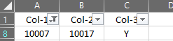
We have three columns below and Col-1 where "Y" is applicable in Col-3 then Col-1 cell value should be base and corresponding Col-2 data should copy against the value. Each corresponding value should paste in the different table (refer the output).

Table 1- Input

Col-1	Col-2	Col-3
10001	10011	Y
10011	10012
10003	10013	Y
10012	10014
10005	10015	Y
10014	10016
10007	10017	Y
10016	10018
10009	10019	Y
10018	10020

Table 2- Output

Output
Col-1	Col-2
10001	10001
10001	10011
10001	10012
10001	10014
10005	10015
10005	10016
10005	10018
10005	10020

Let me know if you need further clarification.

Thank you,

 

[Peter_SSs]

Let me know if you need further clarification.

I don't see how you got the Output table from that Input. Can you explain step-by-step how you got each row in the Output?


BTW, I suggest that you update your Account details (or click your user name at the top right of the forum) so helpers always know what Excel version(s) & platform(s) you are using as the best solution often varies by version. (Don’t forget to scroll down & ‘Save’)

 

[harinsh]

Here is the step by step

1- First filter "Y" in col-3 and take the col-1 cell value (i.e 10001)
2- Paste the above cell value in col-2 and take the value (10011)
3- Paste both above values in empty cells one beside one (10001 - 10011 - Y )

The filter should continue until getting the value incase no value filter should stop and proceed to the second set of data based on value "Y" in Col-3.

 

[Peter_SSs]

Perhaps I am missing something obvious, but I cannot see it.

 

[harinsh]

Here is the step by step

1- First filter "Y" in col-3 and take the col-1 cell value (i.e 10001)
2- Paste the above cell value in col-2 and take the value (10011)
3- Paste both above values in empty cells one beside one (10001 - 10011 - Y )

The filter should continue until getting the value in case no value filter should stop and proceed to the second set of data based on value "Y" in Col-3.

Do you need more clarifications?

 

[Peter_SSs]

That is the same description that you gave before. It makes no sense to me.
Below I have filtered "Y" in col 3.
Why are there four "10001" values in column 1 of the Output?
Where do 10012 and 10014 come from in cells B20 and B21? They seem to have nothing to do with either 10001 in the Input and they also have nothing to do with Y in the Input.

In the Input, the second Y value is for 10003 and 10013. Neither of those values appear in your Output. I don't understand that.

Where do 10016, 10018 and 10020 in cells B23:B26? They seem to have nothing to do with either 10005 in the Input and they also have nothing to do with Y in the Input.

In the Input, the fourth Y value is for 10007 and 10017. Neither of those values appear in your Output. I don't understand that.

In the Input, the fifth Y value is for 10009 and 10019. Neither of those values appear in your Output. I don't understand that.

harnish.xlsm
	A	B	C
1	Table 1- Input
2	Col-1	Col-2	Col-3
3	10001	10011	Y
5	10003	10013	Y
7	10005	10015	Y
9	10007	10017	Y
11	10009	10019	Y
13
14
15	Table 2- Output
16	Output
17	Col-1	Col-2
18	10001	10001
19	10001	10011
20	10001	10012
21	10001	10014
22
23	10005	10015
24	10005	10016
25	10005	10018
26	10005	10020
Sheet1

 

[harinsh]

Need to filter the col-3 value "Y" and take the col-1 value and taking the col-2 value and keeping the values one beside another and take the col-2 value again filtering in col-1 and past beside to the next value.

 

[harinsh]

Below I have filtered "Y" in col 3.

Why are there four "10001" values in column 1 of the Output?
Each "Y" value we call as one set and corresponding hierarchy need to be arranged one after another

Where do 10012 and 10014 come from in cells B20 and B21? They seem to have nothing to do with either 10001 in the Input and they also have nothing to do with Y in the Input.
if you filter 10011 then you get 10012 and if you filter 10012 you will get 10014 and so on..., Input "Y" only to take the set as explained above

In the Input, the second Y value is for 10003 and 10013. Neither of those values appear in your Output. I don't understand that.
Each "Y" value we call as one set and corresponding hierarchy need to be arranged one after another. If you filter 10003 there is no value so this set end with below output

Where do 10016, 10018 and 10020 in cells B23:B26? They seem to have nothing to do with either 10005 in the Input and they also have nothing to do with Y in the Input.
Its hierachy need to align one after one

In the Input, the fourth Y value is for 10007 and 10017. Neither of those values appear in your Output. I don't understand that.
Same as above explained if not further data just make it as one set without hiearchy

In the Input, the fifth Y value is for 10009 and 10019. Neither of those values appear in your Output. I don't understand that.
Same as above explained if not further data just make it as one set without hiearchy

Corrected output

My apologies if any confustion.

 

[Peter_SSs]

OK, no wonder I couldn't understand the (incorrect) original sample and results!
Now I understand.

Try this with a copy of your workbook.

Sub Hierarchy()
  Dim d As Object
  Dim a As Variant, b As Variant, Colm1 As Variant, Colm2 As Variant
  Dim i As Long, j As Long, k As Long
  
  
  Set d = CreateObject("Scripting.Dictionary")
  a = Range("A2", Range("B2").End(xlDown).Offset(, 1)).Value
  For i = 1 To UBound(a)
    d(a(i, 1)) = a(i, 2)
  Next i
  ReDim b(1 To Rows.Count, 1 To 2)
  For i = 1 To UBound(a)
    If a(i, 3) = "Y" Then
      Colm1 = a(i, 1)
      Colm2 = a(i, 2)
      If d.exists(Colm2) Then
        k = k + 1
        Do
          b(k, 1) = Colm1
          b(k, 2) = Colm2
          k = k + 1
          Colm2 = d(Colm2)
        Loop Until IsEmpty(Colm2)
      End If
    End If
  Next i
  If k > 0 Then
    With Range("A1").End(xlDown).Offset(4)
      .Resize(k, 2).Value = b
      .Offset(-1).Resize(, 2).Value = Range("A1:B1").Value
    End With
  End If
End Sub

Sheet before code:

harnish.xlsm
	A	B	C
1	Col-1	Col-2	Col-3
2	10001	10011	Y
3	10011	10012
4	10003	10013	Y
5	10012	10014
6	10005	10015	Y
7	10015	10016
8	10007	10017	Y
9	10016	10018
10	10009	10019	Y
11	10018	10020
12
13
14
15
16
17
18
19
20
Sheet1

After code:

harnish.xlsm
	A	B	C
1	Col-1	Col-2	Col-3
2	10001	10011	Y
3	10011	10012
4	10003	10013	Y
5	10012	10014
6	10005	10015	Y
7	10015	10016
8	10007	10017	Y
9	10016	10018
10	10009	10019	Y
11	10018	10020
12
13
14	Col-1	Col-2
15	10001	10011
16	10001	10012
17	10001	10014
18
19	10005	10015
20	10005	10016
21	10005	10018
22	10005	10020
23
Sheet1

Could you also please address this point I made earlier?

BTW, I suggest that you update your Account details (or click your user name at the top right of the forum) so helpers always know what Excel version(s) & platform(s) you are using as the best solution often varies by version. (Don’t forget to scroll down & ‘Save’)

 

[harinsh]

Wonderfully, you have done what exactly I was looking for only one request, is it possible to add even no hierarchy values as well something like this as one set? So, it will be clear that this value does not have any hierarchy.