Need help with a macro please!

[LuBurt]

Hi,
Can someone please help me, I have some data that needs copying to a new workbook, and there's a lot. I will provide screen shots of examples of what I need to do!

I have one workbook, that shows a list of all customers. There are in total, 744 rows in this workbook, meaning 744 customers.
I have another workbook, that shows all items and the price of that item.
For every customer, I need to copy all items and prices for those items alongside the customers internal ID to a new workbook.
Essentially, this means copying an internal ID from one customer pasting it into a new workbook, copying all items and pricing from another workbook and copying that in to the new workbook. This means I will have to do this for every, single, customer. 744 times.

Here is an example of what I mean.
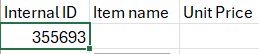
Copy one customer internal ID. For this example, internal ID 355693.

Paste this to a new workbook.

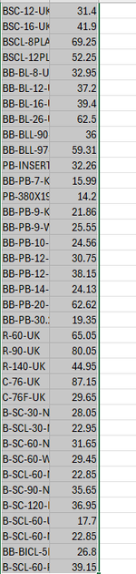
Then, copy all item names and unit prices for those items.

paste to new workbook alongside internal ID.

Autofill internal ID.

This needs to be done for every single customers internal id we have, so 744 times!

Is there ANYTHING I can do to make this faster/automated?

Thanks!

 

[LuBurt]

=LET(a,A2:A4,b,D2:D5,d,D2:E5, ID,VSTACK(a,""), s,VSTACK(0,SEQUENCE(ROWS(a),,ROWS(b),0)), sc,SCAN(1,s,LAMBDA(a,b,a+b)), x,XLOOKUP(SEQUENCE(SUM(ROWS(a)*(ROWS(b)))),sc,ID,,-1), m,TOCOL(MAKEARRAY(ROWS(a),ROWS(b)*2

This is more concise.

=LET(
s,ROUNDUP(SEQUENCE(ROWS(A2:A5)*ROWS(D2:D5))/ROWS(D2:D5),0),
ID,INDEX(A2:A5,s),
Item, INDEX(D2:D5,s),
price, INDEX(E2:E5,s),
HSTACK(ID,Item,price))

I haven't managed to get this to work. For the sake of convenience, I moved everything to one single workbook, as you did so in your example. Not having much luck!

 

[Cubist]

I haven't managed to get this to work. For the sake of convenience, I moved everything to one single workbook, as you did so in your example. Not having much luck!

I don't see what you're putting in so I can't comment. It's most likely you aren't referencing the ranges correctly.

 

[Cubist]

See if the below helps.

=LET(
s,ROUNDUP(SEQUENCE(ROWS(INTERNAL ID)*ROWS(ITEM NAME))/ROWS(ITEM NAME),0),
ID,INDEX(INTERNAL ID,s),
Item, INDEX(ITEM NAME,s),
price, INDEX(PRICE,s),
HSTACK(ID,Item,price))

 

[LuBurt]

I don't see what you're putting in so I can't comment. It's most likely you aren't reference the ranges correctly.

This is probably it, I'm not great with Excel - sorry.

See if the below helps.

=LET(
s,ROUNDUP(SEQUENCE(ROWS(INTERNAL ID)*ROWS(ITEM NAME))/ROWS(ITEM NAME),0),
ID,INDEX(INTERNAL ID,s),
Item, INDEX(ITEM NAME,s),
price, INDEX(PRICE,s),
HSTACK(ID,Item,price))

Sorry, not great with Excel. Let me show you, that might help.

A1 + all of D + E columns.
A1 then duplicates itself to match

Then the same for A2, A3, A4 - until the end (A645)

sorry if im not much help with this, it's painful!

 

[LuBurt]

This is probably it, I'm not great with Excel - sorry.

Sorry, not great with Excel. Let me show you, that might help.

A1 + all of D + E columns.
A1 then duplicates itself to match

Then the same for A2, A3, A4 - until the end (A645)

sorry if im not much help with this, it's painful!





View attachment 110332

We can forget entirely about column B, the company name does NOT need to be there, only the internal id, the price of the item and the item name.

 

[Cubist]

I don't know the last row of your column D and E. Adjust to the last row. Try:

=LET(
a,A1:A645,b,D1:D645,c,E1:E645,
s,ROUNDUP(SEQUENCE(ROWS(a)*ROWS(b))/ROWS(b),0),
ss,MOD(SEQUENCE(ROWS(a)*ROWS(b),,0),ROWS(b))+1,
ID,INDEX(a,s),
Item, INDEX(b,ss),
price, INDEX(c,ss),
HSTACK(ID,Item,price))

 

[LuBurt]

I don't know the last row of your column D and E. Adjust to the last row. Try:

=LET(
a,A1:A645,b,D1:D645,c,E1:E645,
s,ROUNDUP(SEQUENCE(ROWS(a)*ROWS(b))/ROWS(b),0),
ss,MOD(SEQUENCE(ROWS(a)*ROWS(b),,0),ROWS(b))+1,
ID,INDEX(a,s),
Item, INDEX(b,ss),
price, INDEX(c,ss),
HSTACK(ID,Item,price))

Amazing! It worked perfectly. Thank you so much for your help!

 

[Cubist]

Glad that worked out. Cheers.