Primavera P6 Progress Line

[kkqazi]

Hi,
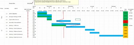
I am looking to make a Gantt Chart where i can show progress as Primavera P6 progress Line does.
I am attaching picture where its like a snake. Any given time, the bar will either move forward or backward depending on status of activity.

any help will be much appreciated.
Thanks

 

[Jeffrey Mahoney]

I could not think of a way to do it with Conditional Formatting. The code below is a way you could add the lines you suggested. I used values of 1 for ahead of schedule, 0 for on schedule, and -1 for behind schedule. It could be triggered automatically when any of your dates are edited or some other way. It basically deletes and recreates all the lines in the range every time.

You should create a named range for the Snake line column.

Sub SnakeLine()

  Dim Cel As Range
  Dim CelHt As Single
  Dim CelLeft As Single
  Dim CelWid As Single
  Dim CelRt As Single
  Dim CelTop As Single
  Dim CelBot As Single
  Dim CelMidVert As Single
  Dim CelMidHorz As Single
  Dim CelVal As Integer
  Dim LastCelVal As Integer
  Dim Node1X As Single
  Dim Node1Y As Single
  Dim Node2X As Single
  Dim Node2Y As Single
  Dim Shp As ShapeRange
  Dim Sht As Worksheet
  Dim X As Long
  Dim Rw As Long
  
  Set Sht = ActiveSheet
  For X = Sht.Shapes.Count To 1 Step -1
    If Left(Sht.Shapes(X).Name, 3) = "Row" Then
      Debug.Print Sht.Shapes(X).Name
      Sht.Shapes(X).Delete
    End If
  Next X
  
    
  For Each Cel In Range("I10:I27")
    CelVal = Cel.Value
    CelLeft = Cel.Left
    CelWid = Cel.Width
    CelRt = CelWid + CelLeft
    CelTop = Cel.Top
    CelHt = Cel.Height
    CelBot = Cel.Top + CelHt
    CelMidVert = CelTop + (CelHt / 2)
    CelMidHorz = CelLeft + (CelWid / 2)
    Rw = Cel.Row
    
    Node1Y = CelTop
    Node2Y = CelBot
    If LastCelVal = 1 And CelVal = 1 Then
      Node1X = CelRt
      Node2X = CelRt
    ElseIf LastCelVal = 0 And CelVal = 1 Then
      Node1X = CelMidHorz
      Node2X = CelRt
    ElseIf LastCelVal = -1 And CelVal = 1 Then
      Node1X = CelLeft
      Node2X = CelRt
    ElseIf LastCelVal = 1 And CelVal = 0 Then
      Node1X = CelRt
      Node2X = CelMidHorz
    ElseIf LastCelVal = 0 And CelVal = 0 Then
      Node1X = CelMidHorz
      Node2X = CelMidHorz
    ElseIf LastCelVal = -1 And CelVal = 0 Then
      Node1X = CelLeft
      Node2X = CelMidHorz
    ElseIf LastCelVal = 1 And CelVal = -1 Then
      Node1X = CelRt
      Node2X = CelLeft
    ElseIf LastCelVal = 0 And CelVal = -1 Then
      Node1X = CelMidHorz
      Node2X = CelLeft
    ElseIf LastCelVal = -1 And CelVal = -1 Then
      Node1X = CelLeft
      Node2X = CelLeft
    End If
    
    ActiveSheet.Shapes.AddConnector(msoConnectorStraight, Node1X, Node1Y, Node2X, Node2Y).Select
    Set Shp = Selection.ShapeRange
    Debug.Print Shp.ID
    Shp.Name = "Row" & Rw
    With Shp.Line
      .Visible = msoTrue
      .Weight = 1.75
      .ForeColor.RGB = RGB(255, 0, 0)
      .Transparency = 0
    End With
  
    LastCelVal = CelVal
  Next Cel
  
  Range("I10").Select
    
End Sub

 

[kkqazi]

I could not think of a way to do it with Conditional Formatting. The code below is a way you could add the lines you suggested. I used values of 1 for ahead of schedule, 0 for on schedule, and -1 for behind schedule. It could be triggered automatically when any of your dates are edited or some other way. It basically deletes and recreates all the lines in the range every time.

You should create a named range for the Snake line column.

Sub SnakeLine()

  Dim Cel As Range
  Dim CelHt As Single
  Dim CelLeft As Single
  Dim CelWid As Single
  Dim CelRt As Single
  Dim CelTop As Single
  Dim CelBot As Single
  Dim CelMidVert As Single
  Dim CelMidHorz As Single
  Dim CelVal As Integer
  Dim LastCelVal As Integer
  Dim Node1X As Single
  Dim Node1Y As Single
  Dim Node2X As Single
  Dim Node2Y As Single
  Dim Shp As ShapeRange
  Dim Sht As Worksheet
  Dim X As Long
  Dim Rw As Long
 
  Set Sht = ActiveSheet
  For X = Sht.Shapes.Count To 1 Step -1
    If Left(Sht.Shapes(X).Name, 3) = "Row" Then
      Debug.Print Sht.Shapes(X).Name
      Sht.Shapes(X).Delete
    End If
  Next X
 
   
  For Each Cel In Range("I10:I27")
    CelVal = Cel.Value
    CelLeft = Cel.Left
    CelWid = Cel.Width
    CelRt = CelWid + CelLeft
    CelTop = Cel.Top
    CelHt = Cel.Height
    CelBot = Cel.Top + CelHt
    CelMidVert = CelTop + (CelHt / 2)
    CelMidHorz = CelLeft + (CelWid / 2)
    Rw = Cel.Row
   
    Node1Y = CelTop
    Node2Y = CelBot
    If LastCelVal = 1 And CelVal = 1 Then
      Node1X = CelRt
      Node2X = CelRt
    ElseIf LastCelVal = 0 And CelVal = 1 Then
      Node1X = CelMidHorz
      Node2X = CelRt
    ElseIf LastCelVal = -1 And CelVal = 1 Then
      Node1X = CelLeft
      Node2X = CelRt
    ElseIf LastCelVal = 1 And CelVal = 0 Then
      Node1X = CelRt
      Node2X = CelMidHorz
    ElseIf LastCelVal = 0 And CelVal = 0 Then
      Node1X = CelMidHorz
      Node2X = CelMidHorz
    ElseIf LastCelVal = -1 And CelVal = 0 Then
      Node1X = CelLeft
      Node2X = CelMidHorz
    ElseIf LastCelVal = 1 And CelVal = -1 Then
      Node1X = CelRt
      Node2X = CelLeft
    ElseIf LastCelVal = 0 And CelVal = -1 Then
      Node1X = CelMidHorz
      Node2X = CelLeft
    ElseIf LastCelVal = -1 And CelVal = -1 Then
      Node1X = CelLeft
      Node2X = CelLeft
    End If
   
    ActiveSheet.Shapes.AddConnector(msoConnectorStraight, Node1X, Node1Y, Node2X, Node2Y).Select
    Set Shp = Selection.ShapeRange
    Debug.Print Shp.ID
    Shp.Name = "Row" & Rw
    With Shp.Line
      .Visible = msoTrue
      .Weight = 1.75
      .ForeColor.RGB = RGB(255, 0, 0)
      .Transparency = 0
    End With
 
    LastCelVal = CelVal
  Next Cel
 
  Range("I10").Select
   
End Sub

Thanks, I will try tomorrow morning. Really appreciate your reply.
Thanks again.

 

[kkqazi]

Hi Jeffrey,
The code does work thank you. however, as i am zero on vba, i have just attached file and also image to show what i would like to do so you can see.
Our business just come up with brilliant idea to use something which require manual intervention and i want something to make it automated.
I want to have that line appear on the day when we review and take data from a column where i will manually input - ( if we are behind ) and + value if we are ahead. 0 will show that we are on plan so it should be straight line.
I wanted to make all this automated but it think it will require so much efforts and conditions.
so i will do all other dates and shading manually, but want progress line to become automated, if possible.
I appreciate your help.

reg
KK

Progress Gantt.xlsx
	A	B	C	D	E	F	G	H	I	J	K	L	M	N	O	P	Q	R	S	T	U	V	W	X	Y
2
3
4
5			Review Date	06/12/2021
6
7	Phase	Line Item	Action		Month	November					December				January					February				RAG Status	Completion Date
8					WK	45	46	47	48	49	50	51	52	53	2	3	4	5	6	7	8	9	10
9				Behind/Ahead (week)	WC	01-Nov	08-Nov	15-Nov	22-Nov	29-Nov	06-Dec	13-Dec	20-Dec	27-Dec	03-Jan	10-Jan	17-Jan	24-Jan	31-Jan	07-Feb	14-Feb	21-Feb	28-Feb
10	Plan	1.1	Define Objective	0	Plan																			GREEN	08-Nov
11					Actual
12		1.2	Arrange meeting with DM	0	Plan																			GREEN	09-Nov
13					Actual
14		1.3	Explore the time line	0	Plan																			GREEN	10-Nov
15					Actual
16		1.4	Assemble Team and Brief	-2	Plan																			RED
17					Actual
18	Do	1.5	Activity 1 - VSM Line	3	Plan																			GREEN	06-Dec
19					Actual
20		1.6	Activity 2 - Identify Hazards	0	Plan																			AMBER
21					Actual
22		1.7	Activity 3 - Measure hazards	0	Plan																			AMBER
23					Actual
24		1.8	Activity 3 - Identify tolerance	0	Plan																			AMBER
25					Actual
26		1.9	Activity 4 - Identify Controls	0	Plan																			AMBER
27					Actual
Sheet1

Cell Formulas
Range	Formula
F8:W8	F8	=WEEKNUM(F9)
G9:W9	G9	=F9+7

 

[Jeffrey Mahoney]

I've done a lot of Gantt Charts, have created tons of automated schedules in Excel, and I have actually worked with Primavera. The method I gave you could easily be updated in seconds, so all we have to do is figure out how you want present the values that drive the lines and where you want to show them. So, do you think this method will work if we can figure those things out?

 

[kkqazi]

Great to hear that. I want to show progress line on chart where we have bars made for progress I.e., plan vs actual. Whole ideas is that any moment of time if I open that chart, I can see if we are on plan, behind plan or ahead of plan. These values either we can generate manually or automatically. Automatic would be great. I had so many automated can’t chart but due to no experience in vba, I got stuck.
I believe status of activity will define the progress bar and where it shows on the chart will depend on the time we open the sheet.
So if I open sheet on 10/12/2021, the line should be on 10/12/21 showing the progress of each activity. Tried to show in picture attached in earlier post.
After your post I feel very positive and excited now.

Reg
KK

 

[Jeffrey Mahoney]

If you want to continue, then lets talk about the line you last created. Normally, a gantt chart is driven by date fields for planned beg, planned end, actual beg, and actual end. I can't see by your snapshot if you have those cells. It looks like you've manually colored the cells instead of having the cells Conditional Formatted to work off the dates provided. In this case, I'm not sure the macro has anything to read to position the lines at the planned beg and end dates if behind or ahead.

Seems to me that a percent complete should be created that compares the number of days completed vs the number of planned days to the review date. As an example:

test.xlsb
	M	N	O	P	Q	R	S	T
1	Planned Beg	Planned End	Planned Days	Expected / Actual Beg	Expected / Actual End	Expected / Actual Days	Days past Deadline	Percent Variance
2	11/26/2021	12/6/2021	10	11/26/2021	12/10/2021	14	4	140%
3	11/26/2021	12/6/2021	10	11/26/2021	12/6/2021	10	0	100%
4	11/26/2021	12/6/2021	10	11/26/2021	12/4/2021	8	-2	80%
Sheet9

Cell Formulas
Range	Formula
R2:R4,O2:O4	R2	=Q2-P2
S2:S4	S2	=Q2-N2
T2:T4	T2	=1+(S2/O2)

 

[Jeffrey Mahoney]

There are several metrics companies use to help manage the budget and time. One is the ratio of actual manhours vs planned manhours. In this case you are only wanting to see the deadline comparison, correct?

 

[kkqazi]

hi
I made this manual just to show in easy way what I wanted. But you are right, a fully automated can’t chart where the bars are generated automatically through given dates in the start and end date.
Ideally I would to see by days. We do not calculate man hours just through days as how far ahead or behind we are.
I used to have Gantt chart which whenever you open it , there is a line showing where we are as we stand. But my manager showed me the example I sent, they wanna see zigzag type line to see ahead and behind plan. Don’t ask why , as we don’t know
So In simple terms.
Start date. End date. How many days has passed and how many completed. If we are behind schedule or ahead of schedule, the line create those snake zig zag showing which activities are ahead or behind.
I think you got it totally right

 

[Jeffrey Mahoney]

So, do you have cells for each line with dates? This macro needs some type of value from which to work. Colored cells are not going to work?