Remove Blanks from a Column with Formula

[IainRourke]

Hi,

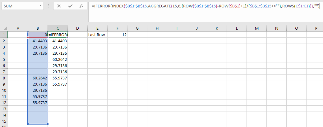
I have a column of data like this:

(COLUMN B)
0
41.44930565
29.71363323
29.71363323



60.26418424
29.71363323
29.71363323



55.97371796
55.97371796

Where the empty cells are actually "" (returned from a previous formula).
What combination of functions should I use if I want to remove the ""s from this list and return the result in a new column? Column C should look like:

(COLUMN C)
0
41.44930565
29.71363323
29.71363323
60.26418424
29.71363323
29.71363323
55.97371796
55.97371796

I think I need to use a combination of INDEX, MATCH and COUNTIF functions, but I don't know the order in which to use them.

Thanks in advance,

Iain

 

[PhilW_34]

Hello,

Is there a reason you can not filter your data and delete the rows that are blank? Then you wouldn't have to put your results into another column. Thanks.

Phil

 

[mgirvin]

Maybe:

<TABLE style="WIDTH: 96pt; BORDER-COLLAPSE: collapse" border=0 cellSpacing=0 cellPadding=0 width=128><COLGROUP><COL style="WIDTH: 48pt" span=2 width=64><TBODY><TR style="HEIGHT: 15pt" height=20><TD style="BORDER-BOTTOM: #f0f0f0; BORDER-LEFT: #f0f0f0; BACKGROUND-COLOR: transparent; WIDTH: 48pt; HEIGHT: 15pt; BORDER-TOP: #f0f0f0; BORDER-RIGHT: #f0f0f0" class=xl65 height=20 width=64 align=right>0





</TD><TD style="BORDER-BOTTOM: windowtext 0.5pt solid; BORDER-LEFT: windowtext 0.5pt solid; BACKGROUND-COLOR: #ccffcc; WIDTH: 48pt; BORDER-TOP: windowtext 0.5pt solid; BORDER-RIGHT: windowtext 0.5pt solid" class=xl67 width=64 align=right>0</TD></TR><TR style="HEIGHT: 15pt" height=20><TD style="BORDER-BOTTOM: #f0f0f0; BORDER-LEFT: #f0f0f0; BACKGROUND-COLOR: transparent; HEIGHT: 15pt; BORDER-TOP: #f0f0f0; BORDER-RIGHT: #f0f0f0" class=xl65 height=20 align=right>41.4493</TD><TD style="BORDER-BOTTOM: windowtext 0.5pt solid; BORDER-LEFT: windowtext 0.5pt solid; BACKGROUND-COLOR: #ccffcc; BORDER-TOP: windowtext; BORDER-RIGHT: windowtext 0.5pt solid" class=xl67 align=right>41.44931</TD></TR><TR style="HEIGHT: 15pt" height=20><TD style="BORDER-BOTTOM: #f0f0f0; BORDER-LEFT: #f0f0f0; BACKGROUND-COLOR: transparent; HEIGHT: 15pt; BORDER-TOP: #f0f0f0; BORDER-RIGHT: #f0f0f0" class=xl65 height=20 align=right>29.7136</TD><TD style="BORDER-BOTTOM: windowtext 0.5pt solid; BORDER-LEFT: windowtext 0.5pt solid; BACKGROUND-COLOR: #ccffcc; BORDER-TOP: windowtext; BORDER-RIGHT: windowtext 0.5pt solid" class=xl67 align=right>29.71363</TD></TR><TR style="HEIGHT: 15pt" height=20><TD style="BORDER-BOTTOM: #f0f0f0; BORDER-LEFT: #f0f0f0; BACKGROUND-COLOR: transparent; HEIGHT: 15pt; BORDER-TOP: #f0f0f0; BORDER-RIGHT: #f0f0f0" class=xl65 height=20 align=right>29.7136</TD><TD style="BORDER-BOTTOM: windowtext 0.5pt solid; BORDER-LEFT: windowtext 0.5pt solid; BACKGROUND-COLOR: #ccffcc; BORDER-TOP: windowtext; BORDER-RIGHT: windowtext 0.5pt solid" class=xl67 align=right>29.71363</TD></TR><TR style="HEIGHT: 15pt" height=20><TD style="BORDER-BOTTOM: #f0f0f0; BORDER-LEFT: #f0f0f0; BACKGROUND-COLOR: yellow; HEIGHT: 15pt; BORDER-TOP: #f0f0f0; BORDER-RIGHT: #f0f0f0" class=xl66 height=20></TD><TD style="BORDER-BOTTOM: windowtext 0.5pt solid; BORDER-LEFT: windowtext 0.5pt solid; BACKGROUND-COLOR: #ccffcc; BORDER-TOP: windowtext; BORDER-RIGHT: windowtext 0.5pt solid" class=xl67 align=right>60.26418</TD></TR><TR style="HEIGHT: 15pt" height=20><TD style="BORDER-BOTTOM: #f0f0f0; BORDER-LEFT: #f0f0f0; BACKGROUND-COLOR: yellow; HEIGHT: 15pt; BORDER-TOP: #f0f0f0; BORDER-RIGHT: #f0f0f0" class=xl66 height=20></TD><TD style="BORDER-BOTTOM: windowtext 0.5pt solid; BORDER-LEFT: windowtext 0.5pt solid; BACKGROUND-COLOR: #ccffcc; BORDER-TOP: windowtext; BORDER-RIGHT: windowtext 0.5pt solid" class=xl67 align=right>29.71363</TD></TR><TR style="HEIGHT: 15pt" height=20><TD style="BORDER-BOTTOM: #f0f0f0; BORDER-LEFT: #f0f0f0; BACKGROUND-COLOR: yellow; HEIGHT: 15pt; BORDER-TOP: #f0f0f0; BORDER-RIGHT: #f0f0f0" class=xl66 height=20></TD><TD style="BORDER-BOTTOM: windowtext 0.5pt solid; BORDER-LEFT: windowtext 0.5pt solid; BACKGROUND-COLOR: #ccffcc; BORDER-TOP: windowtext; BORDER-RIGHT: windowtext 0.5pt solid" class=xl67 align=right>29.71363</TD></TR><TR style="HEIGHT: 15pt" height=20><TD style="BORDER-BOTTOM: #f0f0f0; BORDER-LEFT: #f0f0f0; BACKGROUND-COLOR: transparent; HEIGHT: 15pt; BORDER-TOP: #f0f0f0; BORDER-RIGHT: #f0f0f0" class=xl65 height=20 align=right>60.2642</TD><TD style="BORDER-BOTTOM: windowtext 0.5pt solid; BORDER-LEFT: windowtext 0.5pt solid; BACKGROUND-COLOR: #ccffcc; BORDER-TOP: windowtext; BORDER-RIGHT: windowtext 0.5pt solid" class=xl67 align=right>55.97372</TD></TR><TR style="HEIGHT: 15pt" height=20><TD style="BORDER-BOTTOM: #f0f0f0; BORDER-LEFT: #f0f0f0; BACKGROUND-COLOR: transparent; HEIGHT: 15pt; BORDER-TOP: #f0f0f0; BORDER-RIGHT: #f0f0f0" class=xl65 height=20 align=right>29.7136</TD><TD style="BORDER-BOTTOM: windowtext 0.5pt solid; BORDER-LEFT: windowtext 0.5pt solid; BACKGROUND-COLOR: #ccffcc; BORDER-TOP: windowtext; BORDER-RIGHT: windowtext 0.5pt solid" class=xl67 align=right>55.97372</TD></TR><TR style="HEIGHT: 15pt" height=20><TD style="BORDER-BOTTOM: #f0f0f0; BORDER-LEFT: #f0f0f0; BACKGROUND-COLOR: transparent; HEIGHT: 15pt; BORDER-TOP: #f0f0f0; BORDER-RIGHT: #f0f0f0" class=xl65 height=20 align=right>29.7136</TD><TD style="BORDER-BOTTOM: windowtext 0.5pt solid; BORDER-LEFT: windowtext 0.5pt solid; BACKGROUND-COLOR: #ccffcc; BORDER-TOP: windowtext; BORDER-RIGHT: windowtext 0.5pt solid" class=xl67></TD></TR><TR style="HEIGHT: 15pt" height=20><TD style="BORDER-BOTTOM: #f0f0f0; BORDER-LEFT: #f0f0f0; BACKGROUND-COLOR: yellow; HEIGHT: 15pt; BORDER-TOP: #f0f0f0; BORDER-RIGHT: #f0f0f0" class=xl66 height=20></TD><TD style="BORDER-BOTTOM: windowtext 0.5pt solid; BORDER-LEFT: windowtext 0.5pt solid; BACKGROUND-COLOR: #ccffcc; BORDER-TOP: windowtext; BORDER-RIGHT: windowtext 0.5pt solid" class=xl67></TD></TR><TR style="HEIGHT: 15pt" height=20><TD style="BORDER-BOTTOM: #f0f0f0; BORDER-LEFT: #f0f0f0; BACKGROUND-COLOR: yellow; HEIGHT: 15pt; BORDER-TOP: #f0f0f0; BORDER-RIGHT: #f0f0f0" class=xl66 height=20></TD><TD style="BORDER-BOTTOM: windowtext 0.5pt solid; BORDER-LEFT: windowtext 0.5pt solid; BACKGROUND-COLOR: #ccffcc; BORDER-TOP: windowtext; BORDER-RIGHT: windowtext 0.5pt solid" class=xl67></TD></TR><TR style="HEIGHT: 15pt" height=20><TD style="BORDER-BOTTOM: #f0f0f0; BORDER-LEFT: #f0f0f0; BACKGROUND-COLOR: yellow; HEIGHT: 15pt; BORDER-TOP: #f0f0f0; BORDER-RIGHT: #f0f0f0" class=xl66 height=20></TD><TD style="BORDER-BOTTOM: windowtext 0.5pt solid; BORDER-LEFT: windowtext 0.5pt solid; BACKGROUND-COLOR: #ccffcc; BORDER-TOP: windowtext; BORDER-RIGHT: windowtext 0.5pt solid" class=xl67></TD></TR><TR style="HEIGHT: 15pt" height=20><TD style="BORDER-BOTTOM: #f0f0f0; BORDER-LEFT: #f0f0f0; BACKGROUND-COLOR: transparent; HEIGHT: 15pt; BORDER-TOP: #f0f0f0; BORDER-RIGHT: #f0f0f0" class=xl65 height=20 align=right>55.9737</TD><TD style="BORDER-BOTTOM: windowtext 0.5pt solid; BORDER-LEFT: windowtext 0.5pt solid; BACKGROUND-COLOR: #ccffcc; BORDER-TOP: windowtext; BORDER-RIGHT: windowtext 0.5pt solid" class=xl67></TD></TR><TR style="HEIGHT: 15pt" height=20><TD style="BORDER-BOTTOM: #f0f0f0; BORDER-LEFT: #f0f0f0; BACKGROUND-COLOR: transparent; HEIGHT: 15pt; BORDER-TOP: #f0f0f0; BORDER-RIGHT: #f0f0f0" class=xl65 height=20 align=right>55.9737





</TD><TD style="BORDER-BOTTOM: windowtext 0.5pt solid; BORDER-LEFT: windowtext 0.5pt solid; BACKGROUND-COLOR: #ccffcc; BORDER-TOP: windowtext; BORDER-RIGHT: windowtext 0.5pt solid" id=td_post_2987832 class=xl67></TD></TR></TBODY></TABLE>

In any version of Excel, formula in C1 entered in cell with keystrokes Ctrl + Shift + Enter (not just Entered) and copy down:

=IF(ROWS(C$1:C1)>COUNT($B$1:$B$15),"",INDEX($B$1:$B$15,SMALL(IF($B$1:$B$15<>"",ROW($B$1:$B$15)-ROW($B$1)+1),ROWS(C$1:C1))))

In Excel 2010 use this formula that does not require Ctrl + Shift + Enter:

=IFERROR(INDEX($B$1:$B$15,AGGREGATE(15,6,(ROW($B$1:$B$15)-ROW($B$1)+1)/($B$1:$B$15<>""),ROWS(C$1:C1))),"")

 

[IainRourke]

Thanks, that first formula worked.

Phil: I can't filter the column itself as the values in the column are dynamic. essentialy there are long set of inputs, then many diferent formulas to perform certain opperations on them. then I needed to use a formula to arrange the outputs in a nice way so that they could be graphed. If all goes to plan, I should be able to insert any inputs and get a graph of the outputs.

Thanks again for your help guys.

Iain.

 

[mgirvin]

You are welcome!

 

[mohsen_kh]

@mgirvin
thank you for the reply. Would you please describe me each step of this formula: [ (ROW($B$1:$B$15)-ROW($B$1)+1)/($B$1:$B$15<>"") ] in the following function:

AGGREGATE(15,6,(ROW($B$1:$B$15)-ROW($B$1)+1)/($B$1:$B$15<>""),ROWS(C$1:C1))


Specially I want to know what this part does: ($B$1:$B$15<>"")


It would be of help to me.

Thank you.
Mohsen

 

[damorr]

This is reviving an old thread, but the problem is still current.

In any version of Excel, formula in C1 entered in cell with keystrokes Ctrl + Shift + Enter (not just Entered) and copy down:

=IF(ROWS(C$1:C1)>COUNT($B$1:$B$15),"",INDEX($B$1:$B$15,SMALL(IF($B$1:$B$15<>"",ROW($B$1:$B$15)-ROW($B$1)+1),ROWS(C$1:C1))))

In Excel 2010 use this formula that does not require Ctrl + Shift + Enter:

=IFERROR(INDEX($B$1:$B$15,AGGREGATE(15,6,(ROW($B$1:$B$15)-ROW($B$1)+1)/($B$1:$B$15<>""),ROWS(C$1:C1))),"")

I tried the second formula and it does exactly what I want it to. Except…..

My spreadsheet currently has 40000 rows, and I expect it to grow. I can certainly set the range to be 40000, but then each time I add more data, I have to go through and change all these formulae, a non-trivial and error-prone job.

I tried setting it to 200,000, but this makes Excel crash regularly. It is also glacial whenever I want to do something, like 15 minutes to refresh from the data file.

Is there any way to specify in one place the size of the range so it is easy to update when I have new data?

Thanks

 

[KyleX]

This is reviving an old thread, but the problem is still current.



I tried the second formula and it does exactly what I want it to. Except…..

My spreadsheet currently has 40000 rows, and I expect it to grow. I can certainly set the range to be 40000, but then each time I add more data, I have to go through and change all these formulae, a non-trivial and error-prone job.

I tried setting it to 200,000, but this makes Excel crash regularly. It is also glacial whenever I want to do something, like 15 minutes to refresh from the data file.

Is there any way to specify in one place the size of the range so it is easy to update when I have new data?

Thanks

This is reviving an old thread, but the problem is still current.



I tried the second formula and it does exactly what I want it to. Except…..

My spreadsheet currently has 40000 rows, and I expect it to grow. I can certainly set the range to be 40000, but then each time I add more data, I have to go through and change all these formulae, a non-trivial and error-prone job.

I tried setting it to 200,000, but this makes Excel crash regularly. It is also glacial whenever I want to do something, like 15 minutes to refresh from the data file.

Is there any way to specify in one place the size of the range so it is easy to update when I have new data?

Thanks

I guess this is again reviving an old thread, but hey I managed to find it so maybe this will help someone else...

Your problem can be solved by using the INDIRECT() function. This function allows you to to specify a cell or range (in our case) based on an input. So for example if you have a range $B$1:$B$15 and you would like to change the last row of this range based on an input, then replace that exact segment of the formula with: INDIRECT("$B$1:$B$" & $F$1) where F1 is your input and the last row you'd like the range to go to.

Jumping off of mgirvin's fine solution, you might have something like this (looking into cell C1):

This formula in C1 again is:
=IFERROR(INDEX($B$1:$B$15,AGGREGATE(15,6,(ROW($B$1:$B$15)-ROW($B$1)+1)/($B$1:$B$15<>""),ROWS(C$1:C1))),"")

As you can see, F1 is your input for your last row, so now we will change the formula in C1 to be...

=IFERROR(INDEX(INDIRECT("$B$1:$B$" & $F$1),AGGREGATE(15,6,(ROW(INDIRECT("$B$1:$B$" & $F$1))-ROW($B$1)+1)/(INDIRECT("$B$1:$B$" & $F$1)<>""),ROWS(C$1:C12))),"")

It's a lot longer but all I've done is the copy and pasting I mentioned earlier... any "$B$1:$B$15" turn to "INDIRECT("$B$1:$B$" & $F$1)". This may help with calculation times. And if you'd like to be even more efficent, you can paste this formula into F1, which will calculate your last row # in column B (...or just integrate this into the formula above):

=MAX(ROW(1:65535)*(B1:B65535<>""))

Hope this helps someone!
Kyle

 

[KyleX]

IMPORTANT about my previous post ^ (since I cannot edit my own posts... not sure why that's a thing)

I copied the contents of cell C12 accidentally... What goes into cell C1 as the new substitution should be:

=IFERROR(INDEX(INDIRECT("$B$1:$B$" & $F$1),AGGREGATE(15,6,(ROW(INDIRECT("$B$1:$B$" & $F$1))-ROW($B$1)+1)/(INDIRECT("$B$1:$B$" & $F$1)<>""),ROWS(C$1:C1))),"")

 

[KyleX]

@mgirvin
thank you for the reply. Would you please describe me each step of this formula: [ (ROW($B$1:$B$15)-ROW($B$1)+1)/($B$1:$B$15<>"") ] in the following function:

AGGREGATE(15,6,(ROW($B$1:$B$15)-ROW($B$1)+1)/($B$1:$B$15<>""),ROWS(C$1:C1))


Specially I want to know what this part does: ($B$1:$B$15<>"")


It would be of help to me.

Thank you.
Mohsen

When you have a range like $B$1:$B$15 you are looking at an array. The statement ($B$1:$B$15<>"") tells excel to look through the array $B$1:$B$15 for any cells that are not equal to "" (<> means not equal to and "" refers to blank cells). Again, when you have something like ROW($B$1:$B$15), this tells excel to go through each cell in this range and produce the row number.