Vstack, Chooserows & Dollar

[Nathan Asius]

Hello, I'm hoping someone can help me with this. I think I almost have it.

I am pulling a list of custom user-selected items from a worksheet using a VSTACK function. This is to create a Purchase Order. I have multiple named ranges that are also allow for filtering out blank rows. I this way, no matter how few options, or how many options are selected to be ordered, the list populated by VSTACK appears on another worksheet with no black rows or gaps in the data.

=IF(PanelTotal="","",VSTACK(FILTER(PanelSubPriceToPO,PanelSubPriceToPO<>""))," ")

The Range PanelSubPriceToPO from another worksheet is a single column. The Top row is a header that contains text and proves useful for me to have in the VSTACK. The rest of the column are 16 rows of cells that will contain numbers. VSTACK is very limited in formatting.

However, I managed to find that when I nest the DOLLAR function in the formula, all the numbers convert into the currency format when the result of the VSTACK is displayed.
=IF(PanelTotal="","",VSTACK((DOLLAR(FILTER(PanelSubPriceToPO,PanelSubPriceToPO<>"")))))
The first row in the VSTACK then results to be VALUE# error because the DOLLAR function is applying to the text to it as well.

To solve this, I aimed to separate the first row in the range using the CHOOSEROWS(PanelSubPriceToPO,1) to take the top row and separate it, keeping it as the header in the VSTACK display. The remaining 16 rows with numbers all convert to currency.

=IF(PanelTotal="","",VSTACK(CHOOSEROWS(PanelSubPriceToPO,1),(DOLLAR(FILTER(PanelSubPriceToPO,PanelSubPriceToPO<>"")))))

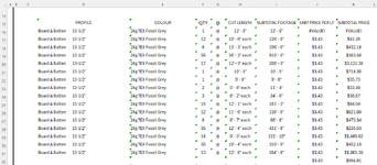
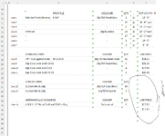
This would work beautifully with the one small snag that the row immediately under the header that I managed to separate, gives me a VALUE# error again. The rest of the cells in the named range are all there but have dropped one row lower. (See image)
No matter where I attempt to place the Chooserows Argument, the FILTER, or the DOLLAR arguments, nor my trial and error with the parentheses, I can not manage to make this work the way I would like.

Is there a problem with my syntax I've overlooked? It seems I'm so close.
Or can I not do what I'm aiming to do with the VSTACK? If so, please suggest a different function that may work better.

Nathan

 

[Nathan Asius]

Thanks for building this.
I had this in ealrier, but for some reason, (I can't figure out why), the named range CustomTrimSubtotalToPO has moved down 4 rows.
There's nothing in the way, and the sheet it's pulling from doesn't seem to be any issues in placements.

 

[Nathan Asius]

...and the last range HASubtotalToPO moved down 8 rows.

 

[StephenCrump]

... but for some reason, ... the named range CustomTrimSubtotalToPO has moved down 4 rows.

We can't tell from a picture.

But on the face of it, it looks like your range StdTrimSubtotlToPO has too many rows? Do you need to filter out the blanks?

 

[Nathan Asius]

I thought it was already filtering out blanks. My original formula using FILTER(StdTrimSubtotlToPO,StdTrimsSubtotlToPO<>"")," "... had this in place.

 

[Nathan Asius]

I would need to insert this argument back into the formula
f,FILTER(v,v<>"")

 

[Nathan Asius]

=IF(PanelTotal="","",VSTACK(FILTER(PanelCutLengthsToPO,PanelCutLengthsToPO<>"")," ",LET(v,VSTACK(StdTrimSubtotlToPO," ",CustomTrimSubtotalToPO," ",HASubtotalToPO," "),f,FILTER(v,v<>""),IFERROR(DOLLAR(v),v))))

This formula did not correct it.

 

[Nathan Asius]

Filtering out blanks for each range in the LET did the trick:

=IF(PanelTotal="","",VSTACK(FILTER(PanelCutLengthsToPO,PanelCutLengthsToPO<>"")," ",LET(v,VSTACK(FILTER(StdTrimSubtotlToPO,StdTrimSubtotlToPO<>"")," ",FILTER(CustomTrimSubtotalToPO,CustomTrimSubtotalToPO<>"")," ",FILTER(HASubtotalToPO,HASubtotalToPO<>"")," "),IFERROR(DOLLAR(v),v))))

 

[StephenCrump]

Filtering out blanks for each range in the LET did the trick

Great, I'm glad you got it working.

You could also filter the three dollar ranges in one go, along these lines:

=IF(PanelTotal="","",LET(p,PanelCutLengthsToPO,v,VSTACK(StdTrimSubtotlToPO," ",CustomTrimSubtotalToPO," ",HASubtotalToPO," "),f,FILTER(v,v<>""),VSTACK(FILTER(p,p<>"")," ",IFERROR(DOLLAR(f),f))))

 

[Nathan Asius]

Thanks Stephen. Yes. That formula works the same though I haven't tested it in all circumstances yet. Testing more maybe will prove it to work better than the one I stumbled to fix.

This leads to a new issue with the #CALC! Empty Array Error.
This formula, I've used to Filter blanks in approx 30 arrays. But in each array there is a header row. What I would like to is if all the other cells in the array are blank, to blank out the header row as well. Ultimately, you see the issue. Filtering out all blanks leads to an Empty Array error.

Other posts here trying to solve the Empty Array error uses VBA. I'm concerned that using a VBA code will need to be duplicated for every one of these 30 or so arrays. Could there be one VBA Code to use that would solve any Empty Array issue on the entire worksheet, rather than tackling each array individually?

The Worksheet is named Purchase Order.