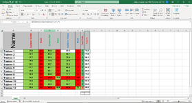
Working out an average of class test results, where resits are capped at 65% and where those not on a resit don't have their average effected.

baileyb103

New Member
Joined
Jan 16, 2023
Messages
22
Office Version
  1. 365
Platform
  1. Windows
I have been asked to produce a spreadsheet where we track trainee test results and to get an average for each trainee. I am currently using the formula =IFERROR(AVERAGEIF(B2:H2,"<>0"),"") so that it doesn't decrease the average for those that don't require a resit. However, for average purposes we want to cap the result at 65%. Ideally for other analysis we want to put in the actual marks scored but have the average work it out as 65% if it is 65% and over. I've been told to just put in 65 and then add a comment of actual score but that wouldn't suit for when they want other analysis conducted.

I've considered putting an IF function in, however unsure as to where it would go, and if there is a better function or method to utilise.

Thank you in advance for any help.
 

Attachments

  • Capture.PNG
    Capture.PNG
    166.3 KB · Views: 7

Excel Facts

Does the VLOOKUP table have to be sorted?
No! when you are using an exact match, the VLOOKUP table can be in any order. Best-selling items at the top is actually the best.
Hi, you could try:

Excel Formula:
=IFERROR(AVERAGE(IF(B2:H2>0,IF(B2:H2>65%,65%,B2:H2))),"")
Thank you. Unfortunately that will generate a flat 65% across the board, whereas I was ideally looking at just col C, E, and G being capped at 65% if over.
 
Upvote 0
Is there something about those columns that we can use to logically determine if they should be capped or not? Something in the header maybe? The screen shot in your first post doesn't appear to be related to the problem at hand.
 
Upvote 0
Apologies, I took the cpature image from the wrong file like a muppet. Here should be the correct image.

It would be columns C, E, and G that would need to be capped at 65%.
 

Attachments

  • Capture.PNG
    Capture.PNG
    106.6 KB · Views: 4
Upvote 0
You could try this:
Excel Formula:
=IFERROR(AVERAGE(IF(B2:H2>0,IF($B$1:$H$1="Resit",IF(B2:H2>65,65,B2:H2),B2:H2))),"")
 
Upvote 0
Solution

Forum statistics

Threads
1,215,069
Messages
6,122,953
Members
449,095
Latest member
nmaske

We've detected that you are using an adblocker.

We have a great community of people providing Excel help here, but the hosting costs are enormous. You can help keep this site running by allowing ads on MrExcel.com.
Allow Ads at MrExcel

Which adblocker are you using?

Disable AdBlock

Follow these easy steps to disable AdBlock

1)Click on the icon in the browser’s toolbar.
2)Click on the icon in the browser’s toolbar.
2)Click on the "Pause on this site" option.
Go back

Disable AdBlock Plus

Follow these easy steps to disable AdBlock Plus

1)Click on the icon in the browser’s toolbar.
2)Click on the toggle to disable it for "mrexcel.com".
Go back

Disable uBlock Origin

Follow these easy steps to disable uBlock Origin

1)Click on the icon in the browser’s toolbar.
2)Click on the "Power" button.
3)Click on the "Refresh" button.
Go back

Disable uBlock

Follow these easy steps to disable uBlock

1)Click on the icon in the browser’s toolbar.
2)Click on the "Power" button.
3)Click on the "Refresh" button.
Go back
Back
Top