Add color in symbol

sksanjeev786

Well-known Member
Joined
Aug 5, 2020
Messages
884
Office Version
  1. 365
  2. 2016
Platform
  1. Windows
Hi Team,

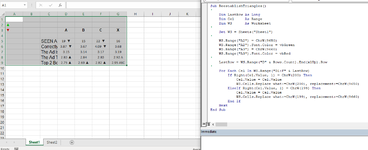
Need to add color in arrow only with Green and Red

01 FS Grouping_Fix Macro.xlsx
ABCDEFGHIJKLMN
1
2
3ABCXABCX
4
5SEEN AD (NET)19 ▼1522 ▼16SEEN AD (NET)19 X1522 X16
6Correctly Branded (net)3.87 ▼3.674.09 ▼3.68Correctly Branded (net)3.87 X3.674.09 X3.68
7The Ad Is Likeable3.153.143.173.19The Ad Is Likeable3.153.143.173.19
8The Ad Told Me Something New2.83 ▲2.842.832.92 AThe Ad Told Me Something New2.832.842.832.92 A
9Top 2 Box (net)2.75 ▲2.69 ▲2.82 ▲2.95 ABCTop 2 Box (net)2.752.692.822.95 ABC
10Top 2 Box (net)2.912.992.84 Top 2 Box (net)2.912.992.84
11
12The Ad Is Likeable3.27 ▼3.23.353.25The Ad Is Likeable3.27 X3.203.353.25
13The Ad Told Me Something New3 ▲2.97 ▲3.04 ▲3.22 ABCThe Ad Told Me Something New3.002.973.043.22 ABC
14It Made Me Want To Visit The Dealership Or Take A Test Drive2.93 ▲2.9 ▲2.97 ▲3.16 ABCIt Made Me Want To Visit The Dealership Or Take A Test Drive2.932.902.973.16 ABC
15The Ad Made Me Want To Find Out More About The Vehicle (search Online/read Articles)3.323.263.37 The Ad Made Me Want To Find Out More About The Vehicle (search Online/read Articles)3.323.263.37
16The Ad Made Me Want To Find Out More About The Brand3.143.153.13 The Ad Made Me Want To Find Out More About The Brand3.143.153.13
17This Is The Sort Of Ad I Would Talk To Others About3.07 ▲3.08 ▲3.05 ▲3.28 ABCThis Is The Sort Of Ad I Would Talk To Others About3.073.083.053.28 ABC
grouping
Cell Formulas
RangeFormula
D5:G10,D12:G17D5=SUBSTITUTE(K5,"X","")&" "&IFERROR(IF(FIND(D$3,$N5),$A$2,""),"")&IFERROR(IF(FIND($G$3,K5),$A$3,""),"")
Cells with Conditional Formatting
CellConditionCell FormatStop If True
K5:M27Expression=FIND($N$3,K5)textNO
K5:M27Expression=FIND(K$3,$N5)textNO
H5:I26Expression=FIND("M",#REF!)textNO
H5:I26Expression=FIND("N",#REF!)textNO


Regards,
Sanjeev
 
The following should return to the triangles that you are used to:

VBA Code:
Sub ReestablishTriangles()
'
    Dim LastRow As Long
    Dim Cel     As Range
    Dim WS      As Worksheet
'
    Set WS = Sheets("Sheet4")                                               ' <--- Change to actual sheet name desired
'
    WS.Range("A2") = ChrW(9650)                                             ' ReEstablish the up Triangle into A2
    WS.Range("A2").Font.Color = vbGreen                                     ' Color the triangle Green
    WS.Range("A3") = ChrW(9660)                                             ' ReEstablish the down Triangle into A3
    WS.Range("A3").Font.Color = vbRed                                       ' Color the triangle Red
'
    LastRow = WS.Range("D" & Rows.Count).End(xlUp).Row                      ' Find the row of the last line of data in Column D
'
    For Each Cel In WS.Range("D1:F" & LastRow)                              ' Range loop
        If Right(Cel.Value, 1) = ChrW(200) Then                             '   If cell ends with a symbol that should be an up triangle then ...
            Cel.Value = Cel.Value                                           '       Remove the formula from the cell to allow a partial color change
            WS.Cells.Replace what:=ChrW(200), replacement:=ChrW(9650)       '       Replace the symbol at the end of the line with an up triangle
        ElseIf Right(Cel.Value, 1) = ChrW(199) Then                         '   If cell ends with a symbol that should be a down triangle then ...
            Cel.Value = Cel.Value                                           '       Remove the formula from the cell to allow a partial color change
            WS.Cells.Replace what:=ChrW(199), replacement:=ChrW(9660)       '       Replace the symbol at the end of the line with a down triangle
        End If
    Next                                                                    ' Loop back
End Sub
 
Upvote 0

Excel Facts

Create a Pivot Table on a Map
If your data has zip codes, postal codes, or city names, select the data and use Insert, 3D Map. (Found to right of chart icons).
The following should return to the triangles that you are used to:

VBA Code:
Sub ReestablishTriangles()
'
    Dim LastRow As Long
    Dim Cel     As Range
    Dim WS      As Worksheet
'
    Set WS = Sheets("Sheet4")                                               ' <--- Change to actual sheet name desired
'
    WS.Range("A2") = ChrW(9650)                                             ' ReEstablish the up Triangle into A2
    WS.Range("A2").Font.Color = vbGreen                                     ' Color the triangle Green
    WS.Range("A3") = ChrW(9660)                                             ' ReEstablish the down Triangle into A3
    WS.Range("A3").Font.Color = vbRed                                       ' Color the triangle Red
'
    LastRow = WS.Range("D" & Rows.Count).End(xlUp).Row                      ' Find the row of the last line of data in Column D
'
    For Each Cel In WS.Range("D1:F" & LastRow)                              ' Range loop
        If Right(Cel.Value, 1) = ChrW(200) Then                             '   If cell ends with a symbol that should be an up triangle then ...
            Cel.Value = Cel.Value                                           '       Remove the formula from the cell to allow a partial color change
            WS.Cells.Replace what:=ChrW(200), replacement:=ChrW(9650)       '       Replace the symbol at the end of the line with an up triangle
        ElseIf Right(Cel.Value, 1) = ChrW(199) Then                         '   If cell ends with a symbol that should be a down triangle then ...
            Cel.Value = Cel.Value                                           '       Remove the formula from the cell to allow a partial color change
            WS.Cells.Replace what:=ChrW(199), replacement:=ChrW(9660)       '       Replace the symbol at the end of the line with a down triangle
        End If
    Next                                                                    ' Loop back
End Sub


Hi johny,

Thanks so much for your time on this


I have just run the macro and looks like getting the same triangle instead of arrow (Wingding 3)

Could you please see the Screenshot I have run the macro but getting trangle
 

Attachments

  • 14.png
    14.png
    43 KB · Views: 4
Upvote 0
That was my fault, it didn't register to me that you wanted to switch from triangles to arrows.

Is there a reason you have all of the symbols reversed in post #20 compared to previous posts?
 
Upvote 0
Try this:

VBA Code:
Sub FlipFlopAndColorArrowsInCells()                                     ' Up triangle = ChrW(9650) ... Down triangle = ChrW(9660) <-- Decimal values of the Hex
'                                                                       ' Up triangle = Unicode Hex 25B2 ... Down triangle = Unicode Hex 25BC
    Dim LastRow As Long
    Dim Cel     As Range
    Dim WS      As Worksheet
'
    Set WS = Sheets("Sheet1")                                                           ' <--- Change to actual sheet name desired
'
    LastRow = WS.Range("D" & Rows.Count).End(xlUp).Row                                  ' Find the row of the last line of data in Column D
'
    WS.Range("A2").Characters(Start:=1, Length:=1).Font.Name = "Wingdings 3"            ' Set character font to Wingdings 3
    WS.Range("A2").Font.Color = vbGreen                                                 ' Color the Arrow Green
'
    WS.Range("A3").Characters(Start:=1, Length:=1).Font.Name = "Wingdings 3"            ' Set character font to Wingdings 3
    WS.Range("A3").Font.Color = vbRed                                                   ' Color the Arrow Red
'
    For Each Cel In WS.Range("D1:F" & LastRow)                                          ' Range loop
        If Right(Cel.Value, 1) = ChrW(199) Then                                         '   If cell should end with an up arrow then ...
            Cel.Value = Cel.Value                                                       '       Remove the formula from the cell to allow a partial color change
            Cel.Value = Replace(Cel.Value, ChrW(199), ChrW(200))                        '       Flip-flop the arrow symbol
            Cel.Characters(Start:=Len(Cel.Value), Length:=1).Font.Name = "Wingdings 3"  '       Set character font to Wingdings 3
            Cel.Characters(Start:=Len(Cel), Length:=1).Font.Color = vbRed               '       Color the arrow Red
'
        ElseIf Right(Cel.Value, 1) = ChrW(200) Then                                     '   If cell should end with a down arrow then ...
            Cel.Value = Cel.Value                                                       '       Remove the formula from the cell to allow a partial color change
            Cel.Value = Replace(Cel.Value, ChrW(200), ChrW(199))                        '       Flip-flop the arrow symbol
            Cel.Characters(Start:=Len(Cel.Value), Length:=1).Font.Name = "Wingdings 3"  '       Set character font to Wingdings 3
            Cel.Characters(Start:=Len(Cel), Length:=1).Font.Color = vbGreen             '       Color the arrow Green
        End If
    Next                                                                                ' Loop back
End Sub

I flip flopped the arrows in the D-F columns to match the data from the previous posts . If you don't want that, just let me know.

Stunning!!! You are absolutely Rockstar of MACRO'S!!!

Thank you So much for your Valuable time and Effort on this......
 
Upvote 0

Forum statistics

Threads
1,215,446
Messages
6,124,896
Members
449,194
Latest member
JayEggleton

We've detected that you are using an adblocker.

We have a great community of people providing Excel help here, but the hosting costs are enormous. You can help keep this site running by allowing ads on MrExcel.com.
Allow Ads at MrExcel

Which adblocker are you using?

Disable AdBlock

Follow these easy steps to disable AdBlock

1)Click on the icon in the browser’s toolbar.
2)Click on the icon in the browser’s toolbar.
2)Click on the "Pause on this site" option.
Go back

Disable AdBlock Plus

Follow these easy steps to disable AdBlock Plus

1)Click on the icon in the browser’s toolbar.
2)Click on the toggle to disable it for "mrexcel.com".
Go back

Disable uBlock Origin

Follow these easy steps to disable uBlock Origin

1)Click on the icon in the browser’s toolbar.
2)Click on the "Power" button.
3)Click on the "Refresh" button.
Go back

Disable uBlock

Follow these easy steps to disable uBlock

1)Click on the icon in the browser’s toolbar.
2)Click on the "Power" button.
3)Click on the "Refresh" button.
Go back
Back
Top