adding two dates which are in text format (3 years 2 months 13 days) + (3 years 4 months 29 days)

myletterboxnp

New Member
Joined
May 20, 2022
Messages
28
Office Version
  1. 365
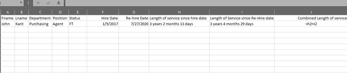
Column F1 has Hire dates (01/09/2017)
Column G1 has re-hire dates (07/27/2020)
Column H1 has calculated length_of_service_Since_Hire (3 years 2 months 13 days) (text field)
Column I1 has calculated length_of_Service_Since_Re_hire (3 years 4 months 29 days) (text filed)

in Column I1, what formula can calculate the seniority date meaning : (Length_of_Service_Since_Hire+Length_of_Service_Since_Re_Hire)?

Some people don't have re_Hire_date.

Thank you!
 
You are not giving us any visibility of what's going on.
Which formula did you try Post #3 or #5.
Can you provide an XL2BB of some sample data ?
At a minimum make you first result in column H the activecell and give us a picture of what your spreadsheet looks like which includes the row and column references and shows the formula bar of the activecell.

Your example uses row 1, is this really the case row 1 is typically a heading row.

Just in case you have extra spaces in your text length of service fields I have added a Trim to the below.
I have also modified it to be in row 2 in case you have headings.
So copy the below into row 2.
If it doesn't work please provide the above information.

Excel Formula:
=LET(arr,TEXTSPLIT(TEXTJOIN(";",TRUE,TRIM(H2),TRIM(I2))," ",";"),
origdays,SUM(--INDEX(arr,0,5)),
origmths,SUM(--INDEX(arr,0,3)) + INT(origdays/31),
fyrs,SUM(--INDEX(arr,0,1))+ INT(origmths/12),
fdays, MOD(origdays,31),
fmths,MOD(origmths,12),
fyrs & " years " & fmths & " months " & fdays & " days  ")
 
Upvote 0

Excel Facts

Bring active cell back into view
Start at A1 and select to A9999 while writing a formula, you can't see A1 anymore. Press Ctrl+Backspace to bring active cell into view.
Could you share the data you are working with? bb code or upload a file somewhere and share the link here?
 
Upvote 0
How about this?:

Excel Formula:
=LET(
a;DIVIDIRTEXTO(H1;" ";;VERDADERO);y_1;ELEGIRCOLS(a;1);m_1;ELEGIRCOLS(a;3);d_1;ELEGIRCOLS(a;5);
b;DIVIDIRTEXTO(I1;" ";;VERDADERO);y_2;SI.ERROR(ELEGIRCOLS(b;1);0);m_2;SI.ERROR(ELEGIRCOLS(b;3);0);d_2;SI.ERROR(ELEGIRCOLS(b;5);0);
y; y_1+y_2+ENTERO((m_1+m_2+ENTERO((d_1+d_2)/30,4375))/12);
m;RESIDUO(m_1+m_2+ENTERO((d_1+d_2)/30,4375);12);
d;ENTERO(RESIDUO(d_1+d_2;30,4375));
t;y & " years " & m & " months " & d & " days";
t)
 
Upvote 0
Sorry ignore last post. Formula is in spanish.
Here is the correcto one:

Excel Formula:
=LET(
    a; TEXTSPLIT(H1; " "; ; TRUE); y_1; CHOOSECOLS(a; 1); m_1; CHOOSECOLS(a; 3); d_1; CHOOSECOLS(a; 5);
    b; TEXTSPLIT(I1; " "; ; TRUE); y_2; IFERROR(CHOOSECOLS(b; 1); 0); m_2; IFERROR(CHOOSECOLS(b; 3); 0); d_2; IFERROR(CHOOSECOLS(b; 5); 0);
    y; y_1 + y_2 + INT((m_1 + m_2 + INT((d_1 + d_2) / 30,4375)) / 12);
    m; MOD(m_1 + m_2 + INT((d_1 + d_2) / 30,4375); 12);
    d; INT(MOD(d_1 + d_2; 30,4375));
    t; y & " years " & m & " months " & d & " days";
    t
)
 
Upvote 0
Hi all,

Here is the sheet.
 

Attachments

  • Service Tenure Test.png
    Service Tenure Test.png
    10.9 KB · Views: 10
Upvote 0
Dave's below formula worked.

=(DATE(INDEX(TEXTSPLIT(H2," ",,1),1),INDEX(TEXTSPLIT(H2," ",,1),3),INDEX(TEXTSPLIT(H2," ",,1),5))+DATE(INDEX(TEXTSPLIT(I2," ",,1),1),INDEX(TEXTSPLIT(I2," ",,1),3),INDEX(TEXTSPLIT(I2," ",,1),5)))/365

Thank you everyone!
 
Upvote 0
The formula calculates but it does it yield the correct answer?

It would really help if you provided an extract of your sheet showing
a) how the text you showed was calculated (3 years 2 months 13 days) and
b) what you want to do with the results for example seniority level is X if months = 84.

I show 2 possible solutions,, Review the suggestions with Excel's formula Evaluation.
N.B. I show the individual calculations for one example below the examples.

You can paste my post to a clean sheet. Click on the icon below the f(x) in the heading, move to your sheet, and paste in cell H1.

T202312a.xlsm
HIJKLMN
1Term with text informationDaysYearsMonths or YearFracor Months
23 years 2 months 13 days3 years 4 months 29 days2,416.1367.46.6279.38
33 years 2 months 13 days3 years 4 months 29 days2,416.1367.46.6279.38
410 years 11 months 13 days3 years 10 months 18 days5,418.441410.014.84178.02
510 years 11 months 13 days3 years 10 months 18 days5,418.441410.014.84178.02
6
74748.25639.1875315418.44
9a
Cell Formulas
RangeFormula
J2,J4J2=LET(a,TEXTSPLIT(H2," ",,1),b,TEXTSPLIT(I2," ",,1),(INDEX(a,1)+INDEX(b,1))*365.25+(INDEX(a,3)+INDEX(b,3))*30.4375+(INDEX(a,5)+INDEX(b,5)))
K2:K5K2=INT(J2/365.25)
L2:L5L2=(J2-K2*365.25)/30.4375
M2:M5M2=YEARFRAC(1,J2,3)
N2:N5N2=J2/30.4375
J3,J5J3=LET(r,H3:I3,SUM(--TEXTBEFORE(r," "))*365.25+SUM(--(RIGHT(TEXTBEFORE(r," ",3),2)))*30.4375+SUM(--(LEFT(TEXTAFTER(r," ",4),2))))
H7H7=SUM(--TEXTBEFORE(H4:I4," "))*365.25
I7I7=SUM(--(RIGHT(TEXTBEFORE(H4:I4," ",3),2)))*30.4375
J7J7=SUM(--(LEFT(TEXTAFTER(H4:I4," ",4),2)))
L7L7=H7+I7+J7
 
Upvote 0
T202312a.xlsm
HIJKLMN
1Term with text informationDaysYearsMonths or YearFracor Months
210 years 11 months 13 days3 years 10 months 18 days5,418.441410.014.84178.02
310 years 11 months 13 days4,000.311011.410.96131.43
43 years 10 months 18 days1,418.13310.63.8846.59
9aa
Cell Formulas
RangeFormula
J2:J4J2=SUM(SUM(TEXTBEFORE(H2," "),IFERROR(TEXTBEFORE(I2," "),0))*365.25,SUM(RIGHT(TEXTBEFORE(H2," ",3),2),IFERROR(RIGHT(TEXTBEFORE(I2," ",3),2),0))*30.4375,SUM(LEFT(TEXTAFTER(H2," ",4),2),IFERROR(LEFT(TEXTAFTER(I2," ",4),2),0)))
K2:K4K2=INT(J2/365.25)
L2:L4L2=(J2-K2*365.25)/30.4375
M2:M4M2=YEARFRAC(1,J2,3)
N2:N4N2=J2/30.4375


T202312a.xlsm
HIP
1Term with text informationMonths
210 years 11 months 13 days3 years 10 months 18 days177
9aa
Cell Formulas
RangeFormula
P2P2=DATEDIF(1,SUM(SUM(TEXTBEFORE(H2," "),IFERROR(TEXTBEFORE(I2," "),0))*365.25,SUM(RIGHT(TEXTBEFORE(H2," ",3),2),IFERROR(RIGHT(TEXTBEFORE(I2," ",3),2),0))*30.4375,SUM(LEFT(TEXTAFTER(H2," ",4),2),IFERROR(LEFT(TEXTAFTER(I2," ",4),2),0))),"M")
 
Last edited:
Upvote 0
A clearly worded question can yield a quality solution.
The source information may yield the most accurate answer.
N.B. We do not know anything about your sheet except what you tell us.
- what are you trying to achieve
- how is your data set up
- is the date information etc. unambiguous
- what version of Excel are you using

Please answer our questions.

I will provide additional information; I hope that my examples are clear.
The information may help you or help others who read the posts.
N.B. I still do not know what you are trying to achieve and the nature of your data.

1. Read the second example first

TextSplit.xlsm
ABC
6Days
73 years 2 months 13 days3 years 4 months 29 days2,416.11
83 years 2 months 13 days3 years 4 months 29 days2,416.11
912 years 10 months 9 days4,696.35
4a
Cell Formulas
RangeFormula
C7C7=(3+3)*365.25+(2+4)*30.4345+(13+29)
C8:C9C8=LET(y,365.25,m,30.435,a,TEXTSPLIT(A8," ",,1),b,TEXTSPLIT(B8," ",,1),INDEX(a,1)*y+INDEX(a,3)*m+INDEX(a,5)+IF(B8>"",INDEX(b,1)*y+INDEX(b,3)*m+INDEX(b,5)))


TextSplit.xlsm
ABCDEFGHI
1
2StartEndDaysStart 2CurrentDaysTotal Days
309-Jan-1727-Jul-20129601-Sep-2023-Dec-2312092505
401-Jan-2331-Dec-233650365
5
4aa
Cell Formulas
RangeFormula
H3:H4H3=(COUNT(F3:G3)=2)*(G3-F3+1)
I3:I4I3=D3+H3
D3:D4D3=C3-B3+1


You can put the Lambda function into your workbook. With Name Manager, name the function to your preference and put the data shown in the Value area.
If you must sum the days worked from the text that you posted; review the following.
You can also build your own function to do this. It does not require VBA and it will work throughout your workbook.
TextSplit.xlsm
ABC
1Days
23 years 2 months 13 days3 years 4 months 29 days2,416.11
312 years 10 months 9 days4,696.35
43 years 6 months 18 days1,296.36
4a
Cell Formulas
RangeFormula
C2C2=SplitToDays(A2,B2)
C3:C4C3=SplitToDays(A3)
Lambda Functions
NameFormula
SplitToDays=LAMBDA(Date1,[Date2],LET(d_1,Date1,d_2,Date2,y,365.25,m,30.435,a,TEXTSPLIT(d_1," ",,1),b,TEXTSPLIT(d_2," ",,1),INDEX(a,1)*y+INDEX(a,3)*m+INDEX(a,5)+IF(d_2>"",INDEX(b,1)*y+INDEX(b,3)*m+INDEX(b,5))))
 
Last edited:
Upvote 0

Forum statistics

Threads
1,215,069
Messages
6,122,959
Members
449,096
Latest member
Anshu121

We've detected that you are using an adblocker.

We have a great community of people providing Excel help here, but the hosting costs are enormous. You can help keep this site running by allowing ads on MrExcel.com.
Allow Ads at MrExcel

Which adblocker are you using?

Disable AdBlock

Follow these easy steps to disable AdBlock

1)Click on the icon in the browser’s toolbar.
2)Click on the icon in the browser’s toolbar.
2)Click on the "Pause on this site" option.
Go back

Disable AdBlock Plus

Follow these easy steps to disable AdBlock Plus

1)Click on the icon in the browser’s toolbar.
2)Click on the toggle to disable it for "mrexcel.com".
Go back

Disable uBlock Origin

Follow these easy steps to disable uBlock Origin

1)Click on the icon in the browser’s toolbar.
2)Click on the "Power" button.
3)Click on the "Refresh" button.
Go back

Disable uBlock

Follow these easy steps to disable uBlock

1)Click on the icon in the browser’s toolbar.
2)Click on the "Power" button.
3)Click on the "Refresh" button.
Go back
Back
Top