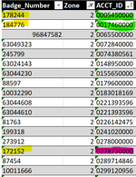
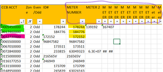
My tables have Badge Numbers and Account IDs. Table 1 has the Badge Numbers pivoted where the row has one Account ID and multiple Badge Numbers across multiple columns. Table 2 has the Badge Numbers unpivoted, so each row has one Badge Number and one Account Number. I would like to apply a conditional formatting to the Account IDs in Table 2 if the Account ID associated to the Badge Number in Table 1 does not match.
In the images below, Table 1 has the Orange header and Table 2 has the black. The lookup value is Table 2 Column A, Lookup Array is Table 1 Columns E:P. The columns to check for match is Column A in Table 1, and Column C in Table 2.
Thanks for looking at my question.
In the images below, Table 1 has the Orange header and Table 2 has the black. The lookup value is Table 2 Column A, Lookup Array is Table 1 Columns E:P. The columns to check for match is Column A in Table 1, and Column C in Table 2.
Thanks for looking at my question.