AverageIF that contain a text for visible/filtered cells only

floW_5

New Member
Joined
Jan 4, 2024
Messages
17
Office Version
  1. 365
Platform
  1. Windows
Sorry, newbie here. I've been looking around (probably not hard enough) for the most appropriate formula with the AVERAGEIF function to work with filtered/visible cells only.

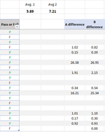
These are the two formula i am using atm which is working perfectly fine to show all data. But not when i filter out certain criteria because it keeps recognizing all cell within the table. Screenshot also attached.
=IFERROR(AVERAGEIF(AA:AA,"P",AD:AD),"")
and
=IFERROR(AVERAGEIF(AA:AA,"P",AE:AE),"")

I am truly sorry if this post have been made many times before me. I have tried a bunch of different solution from here & reddit and maybe I'm inputting something wrong but nothing seems to work for me yet.
 

Attachments

  • Screenshot 2024-01-04 173139.png
    Screenshot 2024-01-04 173139.png
    12.5 KB · Views: 6
Data1.xlsx
ABCDEFGHI
1DATA
2
3Avg1Avg2
45.897.21
5Column4Column5Column21Column22Pass or FailDifference1Difference2
6Day 134.65151.98P  
7Day 241.64448.92F  
8Day 378.79511.20P  
9Day 480.65519.6479.12634.78F1.020.82
10Day 59.84114.1163.95289.90P0.150.39
11Day 631.87261.15P  
12Day 786.01247.723.269.19P26.3826.95
13Day 857.13265.97F  
14Day 9162.82994.8385.39462.84P1.912.15
15Day 10113.72231.42P  
16Day 11131.11879.80F  
17Day 1228.1491.5582.94169.86P0.340.54
18Day 13131.25879.808.1034.73P16.2125.34
19Day 1437.82123.59P  
20Day 1599.3399.43F  
21Day 1647.11227.55P  
22Day 1748.85276.3348.33250.68P1.011.10
23Day 185.2236.8231.29124.21P0.170.30
24Day 1982.23160.0889.06171.89P0.920.93
25Day 2061.49381.22F  
26
27
DATA
Cell Formulas
RangeFormula
G4G4=IFERROR(AVERAGEIF(F6:F1000,"P",G6:G1000),"")
H4H4=IFERROR(AVERAGEIF(F6:F1000,"P",H6:H1000),"")
G6:H25G6=IF(AND(B6<>"",D6<>""),(B6/D6),"")
Cells with Conditional Formatting
CellConditionCell FormatStop If True
F6:F1048576Cell Valuecontains "F"textNO
F6:F1048576Cell Valuecontains "P"textNO


Hope this helps
 
Upvote 0

Excel Facts

How to fill five years of quarters?
Type 1Q-2023 in a cell. Grab the fill handle and drag down or right. After 4Q-2023, Excel will jump to 1Q-2024. Dash can be any character.
Unfortunately post #11 does not answer any of the 3 questions asked in post #10. :(

So, I will assume these answers
It looks like your image shows a formal Excel table at the left with only about 20 rows. Is that the case?
Yes, it is a formal table

If so, what is the name of the table?
Table1

What columns does the entire table occupy?
Columns B:H

IF
those assumptions are correct then could you use this method?

Add a new column to the table as shown below. This column can then be hidden if you want.
Use the average formulas shown in row 4

floW_5.xlsm
ABCDEFGHI
1DATA
2
3Avg1Avg2
45.8868294797.211847711
5Column4Column5Column21Column22Pass or FailDifference1Difference2Vis
6Day 134.645151.976P  1
7Day 241.643448.917F  1
8Day 378.787511.195P  1
9Day 480.648519.64179.117634.779F1.0193510880.8186171881
10Day 59.843114.11463.95289.902P0.1539171230.3936295711
11Day 631.874261.153P  1
12Day 786.014247.723.269.193P26.3846625826.94658981
13Day 857.134265.968F  1
14Day 9162.82994.82985.394462.835P1.9066913372.1494247411
15Day 10113.722231.415P  1
16Day 11131.106879.795F  1
17Day 1228.13991.54682.936169.857P0.3392857140.5389592421
18Day 13131.247879.7958.09734.725P16.2093367925.336069111
19Day 1437.82123.59P  1
20Day 1599.3399.429F  1
21Day 1647.112227.55P  1
22Day 1748.846276.33448.332250.677P1.0106347761.1023508341
23Day 185.21836.82331.288124.214P0.1667732040.2964480651
24Day 1982.234160.08289.062171.889P0.9233343060.9313103221
25Day 2061.488381.223F  1
Sheet1
Cell Formulas
RangeFormula
G4G4=IFERROR(AVERAGEIFS(Table1[Difference1],Table1[Pass or Fail],"P",Table1[Vis],1),"")
H4H4=IFERROR(AVERAGEIFS(Table1[Difference2],Table1[Pass or Fail],"P",Table1[Vis],1),"")
G6:H25G6=IF(AND(B6<>"",D6<>""),(B6/D6),"")
I6:I25I6=SUBTOTAL(3,[@[Pass or Fail]])
 
Upvote 0
The table name is just called "Data" and Yes i believe just a normal table using Ctrl T and pressing enter.
I have tried your method, although it is what i believe you think I am trying to achieve but it is not. I blame myself for not explaining it clear enough. My apologies, English isn't my first language. Ill try my best to explain this again the best I can.

I am just after a formula to input in cell G4 to calculate the average from "Difference1" to only averageIF it contains the letter "P" from "Pass or Fail" column. Atm my formula and your updated one already does that, but as soon as I use the filter to hide certain value. The 5.89 should also change. But in this case, it remains 5.89. With the screenshot also attached, G4 value should now be showing 1.46 just averaging up G14 and G22, excluding G9 because it doesn't contain the "P" from "Pass or Fail".

I really hope this makes sense now. My apologies for the bad interpretation and i do appreciate your time and effort on trying to resolve this. Thank you very much Peter

Data1.xlsx
ABCDEFGHIJ
1
2
3Avg1Avg2
45.897.21
5Column1Column2Column3Column4Column5Pass or FailDifference1Difference2Vis
9Day 1280.65519.6479.12634.78F1.020.821.00
14Day 17162.82994.8385.39462.84P1.912.151.00
22Day 648.85276.3348.33250.68P1.011.101.00
26
27
DATA
Cell Formulas
RangeFormula
G4G4=IFERROR(AVERAGEIFS(Data[Difference1],Data[Pass or Fail],"P",Data[Vis],1),"")
H4H4=IFERROR(AVERAGEIF(F6:F1000,"P",H6:H1000),"")
G9:H9,G14:H14,G22:H22G9=IF(AND(B9<>"",D9<>""),(B9/D9),"")
 

Attachments

  • Screenshot 2024-01-05 203320.png
    Screenshot 2024-01-05 203320.png
    24.5 KB · Views: 2
Upvote 0
In your XL2BB mini sheet in post #14, the 'Vis' column in the table appears to just contain hard-coded 1.00 values. It should contain the formula =SUBTOTAL(3,[@[Pass or Fail]]) as per the mini sheet in post #13

1704449271956.png
 
Upvote 0
In your XL2BB mini sheet in post #14, the 'Vis' column in the table appears to just contain hard-coded 1.00 values. It should contain the formula =SUBTOTAL(3,[@[Pass or Fail]]) as per the mini sheet in post #13

View attachment 104462
Yes! this works. Thank you very much sir you are the greatest 🙏 
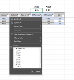
I didn't notice the formula for I6. I am curious though, is there a method to not use the extra Vis column? If not how do you hide the extra column?
 
Upvote 0

Forum statistics

Threads
1,215,077
Messages
6,122,991
Members
449,094
Latest member
masterms

We've detected that you are using an adblocker.

We have a great community of people providing Excel help here, but the hosting costs are enormous. You can help keep this site running by allowing ads on MrExcel.com.
Allow Ads at MrExcel

Which adblocker are you using?

Disable AdBlock

Follow these easy steps to disable AdBlock

1)Click on the icon in the browser’s toolbar.
2)Click on the icon in the browser’s toolbar.
2)Click on the "Pause on this site" option.
Go back

Disable AdBlock Plus

Follow these easy steps to disable AdBlock Plus

1)Click on the icon in the browser’s toolbar.
2)Click on the toggle to disable it for "mrexcel.com".
Go back

Disable uBlock Origin

Follow these easy steps to disable uBlock Origin

1)Click on the icon in the browser’s toolbar.
2)Click on the "Power" button.
3)Click on the "Refresh" button.
Go back

Disable uBlock

Follow these easy steps to disable uBlock

1)Click on the icon in the browser’s toolbar.
2)Click on the "Power" button.
3)Click on the "Refresh" button.
Go back
Back
Top