Blood Pressure Average Formula

[RickyV]

I am trying to figure out how to pick individual cells like E64, E66, E67 skipping E65 rather than a series of cells like (E64:E67) so I want to pick each cell to calculate using CTRL and clicking one by one. MY problem is
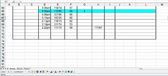
my formula is set up so a series (E66:E70,3)as a 3 place systolic integer and (E66:E70,2)as a 2 place diastolic integer - shown as 111/67 in the pic. The problem is when I pick individual cells there is a comma in between each cell pick like (E64, E66. E67,3) but now the comma in front of the number dictating the places in the systolic and diastolic integer (3 place and 2 place) confuses excel I think because of the commas also between the chosen individual cells and reports an error and will not calculate the average for the individual cells picked. How can I program the ,2 and the ,3 so that it dictates the places for the sys/dia integers so that it is not within the cell choice parenthesis so I can pick and choose individual cells for the average calculation? OR is there a better way to tell the formula the sys/dia are 3 & 2 place integers? I've seen other formylas to calculate this and they are way over complicated so I was hoping to modify my formula a tiny bit to do what I want.
This is the formula and works great when picking a series of cells and rounds the sys/dia to the nearest whole integer:
=ROUND(AVERAGE(VALUE(LEFT(E66:E70,3))),0)&"/"&ROUND(AVERAGE(VALUE(RIGHT(E66:E70,2))),0)

 

[StephenCrump]

Welcome to the Forum!

You'd be better off using the X's in your helper column G to exclude values. You also need to allow for 2-digit systolics and 3 digit diastolics.

So perhaps:

=ROUND(AVERAGE(IF(G64:G70<>"X",--LEFT(E64:E70,FIND("/",E64:E70)-1))),0)&"/"&ROUND(AVERAGE(IF(G64:G70<>"X",--RIGHT(E64:E70,LEN(E64:E70)-FIND("/",E64:E70)))),0)

 

[footoo]

Why not separate the systolic and diastolic numbers into two columns?

 

[sheetspread]

I understand the urge to keep two figures in one cell, but they belong apart. Then your formula will be much simpler.

 

[footoo]

I understand the urge to keep two figures in one cell, but they belong apart. Then your formula will be much simpler.

Including easier to highlight numbers by conditional formatting that are too high / too low.
(Which is more appropriate than the averages.)

 

[RickyV]

Including easier to highlight numbers by conditional formatting that are too high / too low.
(Which is more appropriate than the averages.)

Yeah, 2 columns would be waaay too easy though LOL I want it to look pretty without a lot of monkeying around and yes I am still working on the rest of the Blood Pressure and Heart Rate log sheet and the final will highlight the highs and the lows as well as a weekly/monthly line graph. The 2 digit integer in Column F is the heart rate. The long merged cells to the right are for notes like when large meals are eaten/when medications are taken/types of physical activity etc. so any spikes/lows on the graph chart can be referenced back to the data to see if meds or diet is the possible culprit.

 

[RickyV]

Welcome to the Forum!

You'd be better off using the X's in your helper column G to exclude values. You also need to allow for 2-digit systolics and 3 digit diastolics.

So perhaps:

=ROUND(AVERAGE(IF(G64:G70<>"X",--LEFT(E64:E70,FIND("/",E64:E70)-1))),0)&"/"&ROUND(AVERAGE(IF(G64:G70<>"X",--RIGHT(E64:E70,LEN(E64:E70)-FIND("/",E64:E70)))),0)

Column G is for logging Irregular Heart Beat and that is what the X is.

 

[StephenCrump]

Column G is for logging Irregular Heart Beat and that is what the X is.

Ok, but the comment stands. If you want to pick and choose which values to in/exclude, you're better off using a helper column.

Yeah, 2 columns would be waaay too easy though LOL I want it to look pretty without a lot of monkeying around ....

... but better still to use two different cells, as @sheetspread and @footoo have pointed out. Especially if you're going to do other things like graphing.

If you want pretty, you could do something like this:

	BP
	120	/	80
	125	/	76
		/
		/
		/