Calculate Column G - Column H if Column D is within date range

[DH613]

Hi all,
I thought this would be easy, but I'm having difficulty figuring this out.
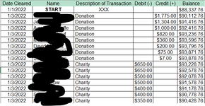
I have a basic transaction register on worksheet "2022" in my workbook. In column D I have the date of the transaction, and I put in the amount in column G if it's a debit, and in column H if it's a credit.
In Sheet 1 I have a list of months (1/1/2022 shown as January 2022, etc.) in column A and wanted to show the total value of credits minus debits for that month in column B.
I wrote - =IF(AND('2022'!D:D>=A2,'2022'!D:D<=A3),SUM('2022'!H:H)-SUM('2022'!G:G)) but that's not working.
What should I be doing?

 

[Fluff]

How about

=SUMIFS('2022'!H:H,'2022'!D:D,">="&A2,'2022'!D:D,"<="&A3)-SUMIFS('2022'!G:G,'2022'!D:D,">="&A2,'2022'!D:D,"<="&A3)

 

[keef2]

This should work

Book1
	A	B	C	D	E	F	G	H	I
1				Date Clear	Name	Descriptoion	Debit	Credit	Balance
2	1/1/2022	$ 1,671.00		1/3/2022		xxx			$ 88,337.76
3	2/1/2022	$ 420.00		1/3/2022		Donation		$ 1,775.00	$ 90,112.76
4	3/1/2022			1/3/2022		Donation		$ 1,304.00	$ 91,416.76
5	4/1/2022			1/3/2022		Donation		$ 1,000.00	$ 92,416.76
6	5/1/2022			2/25/2022		Donation		$ 820.00	$ 93,236.76
7				1/3/2022		Donation		$ 360.00	$ 93,596.76
8				1/3/2022		Donation		$ 200.00	$ 93,796.76
9				1/3/2022		Donation		$ 75.00	$ 93,871.76
10				1/3/2022		Donation		$ 7.00	$ 93,878.76
11				1/3/2022		Charity	$ 650.00		$ 93,228.76
12				1/3/2022		Charity	$ 650.00		$ 92,578.76
13				1/3/2022		Charity	$ 500.00		$ 92,078.76
14				1/3/2022		Charity	$ 500.00		$ 91,578.76
15				1/3/2022		Charity	$ 400.00		$ 91,178.76
16				2/25/2022		Charity	$ 400.00		$ 90,778.76
17				1/3/2022		Charity	$ 350.00		$ 90,428.76
18
19							$ 3,450.00	$ 5,541.00
20								$ 2,091.00
Sheet1

Cell Formulas
Range	Formula
B2:B3	B2	=SUMPRODUCT($H$2:$H$17,--(MONTH($D$2:$D$17)=MONTH($A2)))-SUMPRODUCT($G$2:$G$17,--(MONTH($D$2:$D$17)=MONTH($A2)))
I3:I17	I3	=I2+H3-G3
G19:H19	G19	=SUM(G2:G17)
H20	H20	=H19-G19

 

[DH613]

How about

=SUMIFS('2022'!H:H,'2022'!D:D,">="&A2,'2022'!D:D,"<="&A3)-SUMIFS('2022'!G:G,'2022'!D:D,">="&A2,'2022'!D:D,"<="&A3)

Worked perfectly, thank you

 

[Fluff]

Glad we could help & thanks for the feedback.