Changes in Sorting Order

[Daviboy30]

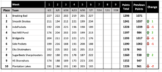
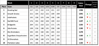
I play in a pool league in which we total the points accumulated each week. I re-sort the teams each week based on the total points. Is there a way to indicate how many places a team has moved up, or down, or stayed the same from the previous week based on the totals?

SLDIPL-LeagueStandings_23529.xlsm
	B	C	D	E	F	G	H	I	J	K	L	M
3		Week	1	2	3	4	5	6	7	8	9	Points Total
4	Place	Team	6/2	6/9	6/16	6/23	6/30	7/7	7/14	7/21	7/28
5	1	Breaking Bad	227	222	202	219	201	227				1298
6	2	Smooth Strokes	211	194	212	221	199	204				1241
7	3	IndePockets	192	228	225	196	198	189				1228
8	4	Red Mill Pond	176	204	202	203	199	213				1197
9	5	Bridgeville	204	211	210	221	171	176				1193
10	6	Side Pockets	199	216	188	191	208	188				1190
11	7	Elks Shotmakers	192	205	182	181	205	213				1178
12	8	SugarBeets Sharpshooters	202	180	191	178	187	222				1160
13	9	HS Shoreshots	174	188	189	173	223	205				1152
14	10	Plantation Lakes	191	186	191	190	203	165				1126
League Standings

Cell Formulas
Range	Formula
M5:M14	M5	=SUM(D5,E5,F5,G5,H5,I5,J5,K5,L5)

 

[Fluff]

How about

Fluff.xlsm
	A	B	C	D	E	F	G	H	I	J	K	L	M	N
1
2
3			Week	1	2	3	4	5	6	7	8	9	Points Total
4		Place	Team	02/06/2023	09/06/2023	16/06/2023	23/06/2023	30/06/2023	07/07/2023	14/07/2023	21/07/2023	28/07/2023
5		1	Breaking Bad	227	222	202	219	201	227				1298	0
6		2	Smooth Strokes	211	194	212	221	199	204				1241	1
7		3	IndePockets	192	228	225	196	198	189				1228	-1
8		4	Red Mill Pond	176	204	202	203	199	213				1197	2
9		5	Bridgeville	204	211	210	221	171	176				1193	-1
10		6	Side Pockets	199	216	188	191	208	188				1190	-1
11		7	Elks Shotmakers	192	205	182	181	205	213				1178	0
12		8	SugarBeets Sharpshooters	202	180	191	178	187	222				1160	2
13		9	HS Shoreshots	174	188	189	173	223	205				1152	0
14		10	Plantation Lakes	191	186	191	190	203	165				1126	-2
Master

Cell Formulas
Range	Formula
M5:M14	M5	=SUM(D5:L5)
N5:N14	N5	=SUMPRODUCT(--((M5-LOOKUP(2,1/(D5:L5<>""),D5:L5))<($M$5:$M$14-INDEX($D$5:$L$14,,MATCH(TODAY(),$D$4:$L$4,1)))))+1-RANK(M5,$M$5:$M$14)

 

[Fluff]

Thinking about it, I've a sneaking feeling that sumproduct doesn't work with lookup functions in earlier versions, so another option with a helper column

Fluff.xlsm
	A	B	C	D	E	F	G	H	I	J	K	L	M	N	O
1
2
3			Week	1	2	3	4	5	6	7	8	9	Points Total	Previous	Change
4		Place	Team	02/06/2023	09/06/2023	16/06/2023	23/06/2023	30/06/2023	07/07/2023	14/07/2023	21/07/2023	28/07/2023		Points
5		1	Breaking Bad	227	222	202	219	201	227				1298	1071	0
6		2	Smooth Strokes	211	194	212	221	199	204				1241	1037	▲ 1
7		3	IndePockets	192	228	225	196	198	189				1228	1039	▼ 1
8		4	Red Mill Pond	176	204	202	203	199	213				1197	984	▲ 2
9		5	Bridgeville	204	211	210	221	171	176				1193	1017	▼ 1
10		6	Side Pockets	199	216	188	191	208	188				1190	1002	▼ 1
11		7	Elks Shotmakers	192	205	182	181	205	213				1178	965	0
12		8	SugarBeets Sharpshooters	202	180	191	178	187	222				1160	938	▲ 2
13		9	HS Shoreshots	174	188	189	173	223	205				1152	947	0
14		10	Plantation Lakes	191	186	191	190	203	165				1126	961	▼ 2
Master

Cell Formulas
Range	Formula
M5:M14	M5	=SUM(D5:L5)
N5:N14	N5	=M5-LOOKUP(2,1/(D5:L5<>""),D5:L5)
O5:O14	O5	=RANK(N5,$N$5:$N$14)-RANK(M5,$M$5:$M$14)

Cells with Conditional Formatting
Cell	Condition		Cell Format	Stop If True
O5:O14	Expression	=O5>0	text	NO
O5:O14	Expression	=O5<0	text	NO

 

[Daviboy30]

Thanks. I got everything to work properly except the conditional formatting. I don't know how you changed the minus symbols to up and down triangles.

SLDIPL-LeagueStandings_23529.xlsm
	B	C	D	E	F	G	H	I	J	K	L	M	N	O
5	1	Breaking Bad	227	222	202	219	201	227				1298	1071
6	2	Smooth Strokes	211	194	212	221	199	204				1241	1037	1
7	3	IndePockets	192	228	225	196	198	189				1228	1039	-1
8	4	Red Mill Pond	176	204	202	203	199	213				1197	984	2
9	5	Bridgeville	204	211	210	221	171	176				1193	1017	-1
10	6	Side Pockets	199	216	188	191	208	188				1190	1002	-1
11	7	Elks Shotmakers	192	205	182	181	205	213				1178	965
12	8	SugarBeets Sharpshooters	202	180	191	178	187	222				1160	938	2
13	9	HS Shoreshots	174	188	189	173	223	205				1152	947
14	10	Plantation Lakes	191	186	191	190	203	165				1126	961	-2
League Standings

Cell Formulas
Range	Formula
M5:M14	M5	=SUM(D5,E5,F5,G5,H5,I5,J5,K5,L5)
N5:N14	N5	=M5-LOOKUP(2,1/(D5:L5<>""),D5:L5)
O5:O14	O5	=RANK(N5,$N$5:$N$14)-RANK(M5,$M$5:$M$14)

Cells with Conditional Formatting
Cell	Condition		Cell Format	Stop If True
O5:O14	Other Type	Icon set		NO
O5:O14	Cell Value	>0	text	YES
O5:O14	Cell Value	<0	text	NO
O5:O14	Cell Value	<0	text	NO
O5:O14	Cell Value	>0	text	NO
O14	Cell Value	>0	text	NO
O14	Cell Value	<0	text	NO

 

[Fluff]

The CF uses custom cell format.
For the -ve values it's
;▼?0;

and the +ve values is
▲?0

 

[Daviboy30]

Thank you! I've got every thing working perfectly now!

SLDIPL-LeagueStandings_230705.xlsm
	B	C	D	E	F	G	H	I	J	K	L	M	N	O
3		Week	1	2	3	4	5	6	7	8	9	Points Total	Change	Previous Week's Totals
4	Place	Team	6/2	6/9	6/16	6/23	6/30	7/7	7/14	7/21	7/28
5	1	Breaking Bad	227	222	202	219	201	227				1298		1071
6	2	Smooth Strokes	211	194	212	221	199	204				1241	▲ 1	1037
7	3	IndePockets	192	228	225	196	198	189				1228	▼ 1	1039
8	4	Red Mill Pond	176	204	202	203	199	213				1197	▲ 2	984
9	5	Bridgeville	204	211	210	221	171	176				1193	▼ 1	1017
10	6	Side Pockets	199	216	188	191	208	188				1190	▼ 1	1002
11	7	Elks Shotmakers	192	205	182	181	205	213				1178		965
12	8	SugarBeets Sharpshooters	202	180	191	178	187	222				1160	▲ 2	938
13	9	HS Shoreshots	174	188	189	173	223	205				1152		947
14	10	Plantation Lakes	191	186	191	190	203	165				1126	▼ 2	961
League Standings

Cell Formulas
Range	Formula
M5:M14	M5	=SUM(D5,E5,F5,G5,H5,I5,J5,K5,L5)
N5:N14	N5	=RANK(O5,$O$5:$O$14)-RANK(M5,$M$5:$M$14)
O5:O14	O5	=M5-LOOKUP(2,1/(D5:L5<>""),D5:L5)

Cells with Conditional Formatting
Cell	Condition		Cell Format	Stop If True
N5:N14	Cell Value	=0	text	NO
N5:N14	Cell Value	<0	text	NO
N5:N14	Cell Value	>0	text	NO

 

[Fluff]

Glad to help & thanks for the feedback.

 

[Peter_SSs]

Given your sample data layout, you could use this simpler form of LOOKUP in column O

=M5-LOOKUP(9^9,D5:I5)