Columns to rows query

[Adrian10]

Good Morning
I have just joined the forum this morning in the hope that somebody could help me with a problem i am having with my excel spreadsheet.
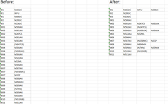
I have a large file that consists of data that looks like this :

0001	N500AX
0002	N501AX
0002	N247CS
0002	N501AX
0003	N502AX
0003	(N247CS)
0004	N504AX
0004	(N500AX)
0004	N504AX

What i need to do is convert the data so it looks like this :-

0001 N500AX
0002 N501AX N247CS N501AX
0003 N502AX (N247CS)
0004 N504AX (N500AX) N504AX

and so on, i realise i can select each serial number individually and use convert to row, but i have 500,000 rows !!

is there a VBA or macro Solution for this ? I attach a image to better illustrate what i am trying to achieve

Any help would be much appreciated

Regards

Adrian

 

[etaf]

as you have 365 version

use
=UNIQUE(A1:A9)
to pull out all the reference numbers
and then
=TEXTJOIN(" ",,FILTER($B$1:$B$9,$A$1:$A$9=D1))
and copy down for the strings

Book6
	A	B	C	D	E
1	0001	N500AX		0001	N500AX
2	0002	N501AX		0002	N501AX N247CS N501AX
3	0002	N247CS		0003	N502AX (N247CS)
4	0002	N501AX		0004	N504AX (N500AX) N504AX
5	0003	N502AX
6	0003	(N247CS)
7	0004	N504AX
8	0004	(N500AX)
9	0004	N504AX
Sheet1

Cell Formulas
Range	Formula
D1:D4	D1	=UNIQUE(A1:A9)
E1:E4	E1	=TEXTJOIN(" ",,FILTER($B$1:$B$9,$A$1:$A$9=D1))
Dynamic array formulas.

 

[Adrian10]

Many many thanks for the swift reply, that works perfectly

Best Regards

Adrian

 

[etaf]

you are welcome

 

[Fluff]

Another option if you want the col B vales in their own cells is.

Fluff.xlsm
	A	B	C	D	E	F	G	H	I
1
2	0001	N500AX			0001	N500AX
3	0002	N501AX			0002	N501AX	N247CS	N501AX
4	0002	N247CS			0003	N502AX	(N247CS)
5	0002	N501AX			0004	N504AX	(N500AX)	N504AX
6	0003	N502AX
7	0003	(N247CS)
8	0004	N504AX
9	0004	(N500AX)
10	0004	N504AX
11
Main

Cell Formulas
Range	Formula
E2:E5	E2	=UNIQUE(FILTER(A2:A100,A2:A100<>""))
F2,F5:H5,F4:G4,F3:H3	F2	=TOROW(FILTER($B$2:$B$100,$A$2:$A$100=E2))
Dynamic array formulas.

 

[Adrian10]

Hi fluff,

I used etaf's method as described in their post, then I highlighted the results, then did text to columns delimited by space, this method is far quicker !!

Many Thanks

 

[Fluff]

Not sure how that's quicker than a formula that does it all, but as long as your happy, that's fine

 

[etaf]

I used etaf's method as described in their post,

Thanks , I tried Fluff when he posted , as i do with most of Fluff replies, and other members , i learn so much stuff that way
It should be much easier , all done in 1 go
anyway -
you are welcome and glad to have helped and provided a solution

 

[alansidman]

A third option is to use Power Pivot as demonstrated in this link

https://sfmagazine.com/articles/2018/july/excel-reporting-text-in-a-pivot-table/?psso=true