Conditional Formatting based on age range

CMW

New Member
Joined
Dec 20, 2023
Messages
9
Office Version
  1. 365
Platform
  1. Windows
Hi
I have a list of names and dates of birth and have a separate column that calculates the age (at a given date) based on the date of birth, giving the answer in X Years, X Months.

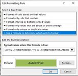
I am trying to use conditional formatting to highlight the names that fall within a set age range for example all those who are between 8 years and 0 months and 9 years and 6 months at the given date. I thought I had cracked it, but when I looked at my results the conditional formatting was also highlighting cells where the age is 9 years, 11 months. Not sure where I have gone wrong or what the solution is (if there is one!).

TIA
 
Select the range: D3:D13
Go to conditional formatting
Use the formula option
Input the below formula:
Excel Formula:
=LET( y,--TEXTBEFORE(D3," Y"), m,--TEXTBEFORE(TEXTAFTER(D3,", ")," M"), AND(y>=8,m>=0,y<=9,m<=6))
Set a format
Click OK
 
Upvote 0

Excel Facts

Copy formula down without changing references
If you have =SUM(F2:F49) in F50; type Alt+' in F51 to copy =SUM(F2:F49) to F51, leaving the formula in edit mode. Change SUM to COUNT.
Dont know where I am going wrong, but it's not working!:cry:
 

Attachments

  • Sample image 3.JPG
    Sample image 3.JPG
    37.4 KB · Views: 4
Upvote 0
Looks like you are doing it right, I am using Excel online at the moment because I don't have access to my laptop but it shouldn't make a difference.

Are you doing this in Excel 365?
 
Upvote 0
How about you count the total month and use this formula in your CF:

Libro1
CDE
101/01/2024
2Date of birthFormula for CF
32013-06-1410 Years, 6 Month0
42013-06-1410 Years, 6 Month0
52012-06-1711 Years, 6 Month0
62014-11-019 Years, 2 Month1
72012-11-1111 Years, 1 Month0
82014-05-229 Years, 7 Month0
92014-05-309 Years, 7 Month0
102015-03-098 Years, 9 Month1
112015-01-228 Years, 11 Month1
122015-03-158 Years, 9 Month1
132013-09-2710 Years, 3 Month0
Hoja1
Cell Formulas
RangeFormula
D3:D13D3=DATEDIF(C3,$D$1,"Y")&" Years, "&DATEDIF(C3,$D$1,"YM")&" Month"
E3:E13E3=LET(m,ROUND(($D$1-C3)/30.4375,0), (m>=96)*(m<=114) )


Why divided by 30,4375 you ask? That number of days comes from dividing a century worth of days in 100 and then in 12. So you get the average number of days per month. And with this you can have a hundred years of date difference and the number of month calculated will be correct.
 
Last edited:
Upvote 0
Hi - for some reason that formula didn't work either (just got a NAME error!). Not to worry, you put me onto another solution so I have found a work around.

Thanks for all you time and help though!
 
Upvote 0
Maybe you are using it on an older version of excel that does not support the functions we used?
 
Upvote 0
Possibly! Thank you again for your time you helped me to find a very good work-around.

Merry Christmas!
 
Upvote 0

Forum statistics

Threads
1,215,069
Messages
6,122,959
Members
449,096
Latest member
Anshu121

We've detected that you are using an adblocker.

We have a great community of people providing Excel help here, but the hosting costs are enormous. You can help keep this site running by allowing ads on MrExcel.com.
Allow Ads at MrExcel

Which adblocker are you using?

Disable AdBlock

Follow these easy steps to disable AdBlock

1)Click on the icon in the browser’s toolbar.
2)Click on the icon in the browser’s toolbar.
2)Click on the "Pause on this site" option.
Go back

Disable AdBlock Plus

Follow these easy steps to disable AdBlock Plus

1)Click on the icon in the browser’s toolbar.
2)Click on the toggle to disable it for "mrexcel.com".
Go back

Disable uBlock Origin

Follow these easy steps to disable uBlock Origin

1)Click on the icon in the browser’s toolbar.
2)Click on the "Power" button.
3)Click on the "Refresh" button.
Go back

Disable uBlock

Follow these easy steps to disable uBlock

1)Click on the icon in the browser’s toolbar.
2)Click on the "Power" button.
3)Click on the "Refresh" button.
Go back
Back
Top