nicolews
New Member
- Joined
- Jun 12, 2015
- Messages
- 7
Hello. I am unable to find the proper conditional formatting custom formula for the below. Help!
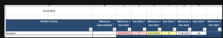
I have a tracker file that shows project milestone due dates and their day count down to those due dates in the next column. The day count down is auto calculated each time you open the file- I’m good there.
Ex: Row 1 shows Project description, milestone #1 due date, milestone #1 day count down, milestone #2 due date, milestone #2 day count down, and so on through milestone #20 due date and it’s day countdown.
What I’m wanting is to add a column before milestone #1 due date that will show me if any of the milestones are approaching (since it’s a lot to scroll continuously to the right and view the due dates/day counters that are already rendered warning colors based on their individual values).
Wanting the new column to display the below if any of the milestones are in range- thinking of using each day count down, but not married to that idea.
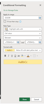
- “Incoming” w/ cell filled yellow: due in 8-15 days
- “Due” cell filled red: due in 0-7 days
- “Past Due” cell filled red w/red bold font: past due date (or a negative day count number)
I understand how to format the new cell based on the value of a different cell… what is tripping me up is how to look for that value across a row and/or in alternating cells in that row. Does that make sense?
I have a tracker file that shows project milestone due dates and their day count down to those due dates in the next column. The day count down is auto calculated each time you open the file- I’m good there.
Ex: Row 1 shows Project description, milestone #1 due date, milestone #1 day count down, milestone #2 due date, milestone #2 day count down, and so on through milestone #20 due date and it’s day countdown.
What I’m wanting is to add a column before milestone #1 due date that will show me if any of the milestones are approaching (since it’s a lot to scroll continuously to the right and view the due dates/day counters that are already rendered warning colors based on their individual values).
Wanting the new column to display the below if any of the milestones are in range- thinking of using each day count down, but not married to that idea.
- “Incoming” w/ cell filled yellow: due in 8-15 days
- “Due” cell filled red: due in 0-7 days
- “Past Due” cell filled red w/red bold font: past due date (or a negative day count number)
I understand how to format the new cell based on the value of a different cell… what is tripping me up is how to look for that value across a row and/or in alternating cells in that row. Does that make sense?
Attachments
Last edited: