Conditional Formatting Every 4 years From Start Date

[94mustang]

Hello Excel Experts,

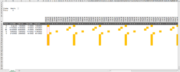
See the uploaded images of my spreadsheet attached this thread. I am wanting to highlight the cell that occurs every 4 years from the Cert Date (Col B) or a start date. The Display (cell B4) will change the dates in the grey header cells from Monthly to Quarterly. The idea is to have the cell in that row to be highlighted in January or the First quarter every 4th year in the future. In my screenshot, I have a custom formula for conditional formatting that is highlighting every January, but I am needing it to be every 4th year.

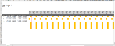
I also upload a screenshot with Display changed to Quarterly and the current formula is working but again the highlighted cell needs to be the first quarter every 4th year.

Likewise, the Surv Date (Col D) occurs every 6 months. I would like a formula that will do this for me as well. Based on any solutions that will resolve my dilemma, I may be able to apply it to the Surv Date for every 6th month in the future.

Any help or advice would be greatly appreciated. Thank you

 

[Micron]

With respect to 2023, 2027, 2031 Year([a date goes here]) Mod 4 will (I think) always return 3. So your CF rule could probably make use of that. Not sure if that approach would be applicable to your other issue. I couldn't make sense of it.

 

[94mustang]

Micron,

Do you have an example formula you could share? You are correct that I would like to highlight the cell in 2023, 2027, 2031 but in January of those years. I know I need to compare the Cert Date to each header date in grey highlight. What would that formula look like to highlight the cell. I think with just a bit more guidance, I can figure out the rest of what I need. It's the first part of just highlighting the corresponding cells.

 

[Micron]

It's hard to suggest anything definitive when you don't really follow. F'rinstance I have no idea why or what the comparison is re:

I know I need to compare the Cert Date to each header date in grey highlight.

If only for January, then you'd use what I showed but only in January cells? Something like if using <Expression> option
Year(Date) Mod 4 = 3 and the cell should be coloured where that is true? If not Date function, then a cell reference?

 

[94mustang]

Hello Micron,

Let me see if I can clarify with a bit more detail. Col A is a manufacturing facility (15, 4, 80, etc), and each row is an independent record. For Plant 15 (first Mfg Plant), the Certification Audit occurred on Jan 2, 2023 (arbitrary date is just an example date). Once that date is entered, I would like to highlight the cells in the row that is 4, 8, 12, etc. years in the future to indicate when the next Certification Audit is to be completed. However, the header dates (grey cells; Col G and beyond) need to be compared to the Cert Date month and year in Col B. There are no formulas in the cells that have the yellow highlight background. It is purely conditional formatting. The idea is when there are many manufacturing facilities, it would be nice just to add the facility and its Certification Date and the table to the right simply populates without having to add formulas to the cells.

I am not able to understand your formula for the conditional formatting rule for both dates (Cert Date comparison to future dates (Col G and beyond)) to be considered to know which cell to highlight with the yellow background. I hope this explanation will provide the necessary clarity. Thank you for your patience.

 

[Micron]

I can get a Mod formula to return 3, but seeing as how it's in a cell formatted as date it's returning 01/03/00, which I think is 1900, not 2000. If I wrap that in Text function, I can return 3 but in a CF rule, neither =3 or ='3' is working. I'll keep trying, but perhaps somebody who is better at this than me will chime in.

 

[Micron]

I must have spent an hour trying to figure out why something would not work. Turns out that somehow calculation got set to manual. I'll bet I had it working in the first 10 minutes. lf B11 contains 1/02/2026 this cf formula works:
=MOD(YEAR(B11),4)=3
I imagine you'd put that against H10, L10 and so on. A lot of formatting if you want this to work for a lot of rows. Looks like it would be at least for rows 10 to 21.
An alternative might be to loop over a range and apply cf using the same logic.