Conditional Formatting Issue

jhculbert

New Member
Joined
Jun 14, 2023
Messages
7
Office Version
  1. 365
Platform
  1. MacOS
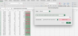
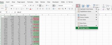
What follows is a Mini-Sheet for a set of data I have, where the specific conditional formatting I want is not working. What I want is for Column F data to show a green background when the data are less than or equal to Column A data, and Red (it actually shows up as pink, as red does not seem to be a background color choice here) when Column F is greater than Column A. What is maddening is I have this same conditional formatting on another block of data in the same spreadsheet, and it is working correctly. I hope someone can help me here. Thanks!

Conditionap_Formatting.xlsx
ABCDEF
2$92.29$3.10735.023.0$96.19
3$566.47$11.4913.150.029.9$519.16
4$80.74$5.783.910.88.5$57.95
5$137.49$103.8414.030.028.8$3,480.30
6$177.51$51.1215.050.086.9$4,024.04
7$178.26$5.629.625.819.6$139.82
8$50.93$3.5810.515.57.0$44.50
9$372.86$26.9312.012.08.4$307.65
10$79.09$3.292.022.017.0$65.44
11$744.11$11.639.735.027.2$396.78
12$122.77$2.715.130.032.6$89.15
13$412.22$8.9412.730.039.5$350.12
14$152.51$5.255.829.118.3$131.64
15$112.83$7.475.615.014.8$117.54
16$66.35$2.118.226.013.2$44.75
17$209.21$8.0110.923.010.0$146.57
18$134.67$3.908.625.027.0$110.12
19$115.13$8.6010.015.07.4$105.95
20$429.29$10.509.730.019.0$282.20
21$283.57$5.2114.032.024.5$167.79
Sheet1
Cell Formulas
RangeFormula
F2:F21F2=(((D2+E2)/2)*B2*(1+(C2/100)))
Cells with Conditional Formatting
CellConditionCell FormatStop If True
F2:F21Cell Value<="Cell Value <= $A$2"textNO
F2:F21Cell Value>"Cell Value <= $A$2"textNO
 

Excel Facts

What did Pito Salas invent?
Pito Salas, working for Lotus, popularized what would become to be pivot tables. It was released as Lotus Improv in 1989.
you have "" around the formula
and not sure about the formula

you have = for both - only 1 needs the =

BUT TRY

for 2007, 2010 , 2013 , 2016 , 2019 or 365 Subscription excel version
Conditional Formatting

Highlight applicable range >>
F1:F100 - Change, reduce or extend the rows to meet your data range of rows

Home Tab >> Styles >> Conditional Formatting
New Rule >> Use a formula to determine which cells to format
Edit the Rule Description: Format values where this formula is true:
=AND($F1<>"",$F1<=$A1)

Format [Number, Font, Border, Fill] - Fill Green
choose the format you would like to apply when the condition is true
OK >> OK

another rule
=$F1>$A1 = Fill RED

Not - I have selected from row 1 - and the formula starts in row 1
so whereever you start the selection to colour make sure the rows are same

so if it starts in row2 - select F2:F100 or howver many rows
and formula
=AND($F2<>"",$F2<=$A2)

Book3
ABCDEF
2566.4711.4913.15029.957.952303
380.745.783.910.88.53480.30144
4137.49103.84143028.84024.0386
5177.5151.12155086.9139.821104
6178.265.629.625.819.644.503875
750.933.5810.515.57307.64832
8372.8626.9312128.465.4381
979.093.2922217396.777221
10744.1111.639.73527.289.148973
11122.772.715.13032.6350.119455
12412.228.9412.73039.5131.64165
13152.515.255.829.118.3117.535968
14112.837.475.61514.844.747192
1566.352.118.22613.2146.570985
16209.218.0110.92310110.1204
17134.673.98.62527105.952
18115.138.610157.4282.20325
19429.2910.59.73019167.78805
20283.575.21143224.50
21
22
23
24
25
Sheet1
Cell Formulas
RangeFormula
F2:F20F2=(((D3+E3)/2)*B3*(1+(C3/100)))
Cells with Conditional Formatting
CellConditionCell FormatStop If True
F1:F100Expression=$F1>$A1textYES
F1:F100Expression=AND($F1<>"",$F1<=$A1)textYES
 
Last edited:
Upvote 0
etaf - Thank you for your quick reply.
You provide alot of varying info. I need to absorb before I can try any of your suggestions.
I'm keeping my fingers crossed I can fix my issue using part of them, at least.
 
Upvote 0
you are welcome
post back anything not understanding or not working
 
Upvote 0
I have now gone through your instructions, and they are quite different than my for my Microsoft for iMac v. 16.83, Office Home & Student 2021. I tried to interpret what you are saying, but all cells in column F remain green, even though my formula set conditions on some becoming pink, when true.

I still need help on my issue. I could share the data section that does work, if that would help.
 
Upvote 0
ok,
i'm also using 365 on a mac

a couple of images

where are you stuck
 

Attachments

  • Screenshot 2024-03-23 at 14.47.20.jpeg
    Screenshot 2024-03-23 at 14.47.20.jpeg
    94.8 KB · Views: 4
  • Screenshot 2024-03-23 at 14.46.36.jpeg
    Screenshot 2024-03-23 at 14.46.36.jpeg
    61.5 KB · Views: 4
Upvote 0
Solution
Well, thank you! Sorry for the delay in responding.
Once I changed the conditional formatting rule for the first row after reviewing your screenshots,
all of the other rows self-corrected.
I don't understand why that would be, but I'm happy it now works for this data section.
 
Upvote 0

Forum statistics

Threads
1,215,140
Messages
6,123,269
Members
449,093
Latest member
Vincent Khandagale

We've detected that you are using an adblocker.

We have a great community of people providing Excel help here, but the hosting costs are enormous. You can help keep this site running by allowing ads on MrExcel.com.
Allow Ads at MrExcel

Which adblocker are you using?

Disable AdBlock

Follow these easy steps to disable AdBlock

1)Click on the icon in the browser’s toolbar.
2)Click on the icon in the browser’s toolbar.
2)Click on the "Pause on this site" option.
Go back

Disable AdBlock Plus

Follow these easy steps to disable AdBlock Plus

1)Click on the icon in the browser’s toolbar.
2)Click on the toggle to disable it for "mrexcel.com".
Go back

Disable uBlock Origin

Follow these easy steps to disable uBlock Origin

1)Click on the icon in the browser’s toolbar.
2)Click on the "Power" button.
3)Click on the "Refresh" button.
Go back

Disable uBlock

Follow these easy steps to disable uBlock

1)Click on the icon in the browser’s toolbar.
2)Click on the "Power" button.
3)Click on the "Refresh" button.
Go back
Back
Top