Countifs to a criteria range that is a derived value

kattay

New Member
Joined
May 28, 2023
Messages
3
Office Version
  1. 2019
Platform
  1. Windows
Hi, I have a roster made from the Excel calendar template. The dates have been pre-populated by formula (see E3). I would like to count the number of "Y" in the calendar (eg. row 4 & row 7), until the effective date, but the countifs does not work on the derived value in the criteria range. My formula is COUNTIFS(B4:H4,"Y",B3:H3,"<"&L2)+COUNTIFS(B7:H7,"Y",B6:H6,"<"&L2).
1685287178186.png

Pls help. Thanks
 

Attachments

  • 1685286772821.png
    1685286772821.png
    31.7 KB · Views: 5
  • 1685286829182.png
    1685286829182.png
    30.6 KB · Views: 5

Excel Facts

Can a formula spear through sheets?
Use =SUM(January:December!E7) to sum E7 on all of the sheets from January through December
What is happening in E4 to make that a Y - is it just typed in by the individual as a value, or is it a formula itself?
 
Upvote 0
I get it to work with the numbers entered manually, but it seems to not like them being the result of a formula. I'm afraid I don't know why. I hope someone much wiser than me will come along soon, but I will keep fiddling with it in the meantime to see if what I can do.
 
Upvote 0
@RachelN76 , you can use SUMPRODUCT function to acheive this. But, can you post data in a table, and not images? It is time consuming and error prone to make the forum recreate your scenario.
 
Upvote 0
Hi @awoohaw, it's my table. Pls see below. Thanks

Calendar sample.xlsx
BCDEFGHIJKL
1June 2023Day
2MONDAYTUESDAYWEDNESDAYTHURSDAYFRIDAYSATURDAYSUNDAYEffective Date of Change:8/6/20238
32930311234
4YYYOld Shift Pattern:(Select One)
5YYYNew Shift Pattern:(Select One)
6567891011
7YYYYNo. of working days (until effective date of change):0
8YYYYNo. of working days (from effective date of change):0
912131415161718
10YYYYNo. of working days in the month (assume full month roster):17
11YYYNo. of working days in the month (assume full month roster):16
1219202122232425
13YYY
14YYY
15262728293012
16YYY
17YYY
June
Cell Formulas
RangeFormula
B1B1="June "&CalendarYear
B2B2=IF(WeekStart="SUNDAY", "SUNDAY","MONDAY")
C2:H2C2=UPPER(TEXT(C3,"dddd"))
B3:H3B3=DaysAndWeeks+DATE(CalendarYear,6,1)-WEEKDAY(DATE(CalendarYear,6,1),(WeekStart="Monday")+1)+1
L2L2=DAY(K2)
B6:H6B6=DaysAndWeeks+DATE(CalendarYear,6,1)-WEEKDAY(DATE(CalendarYear,6,1),(WeekStart="Monday")+1)+8
K7K7=COUNTIFS(B4:H4,"Y",B3:H3,"<"&L2)++COUNTIFS(B7:H7,"Y",B6:H6,"<"&L2)+COUNTIFS(B10:H10,"Y",B9:H9,"<"&L2)+COUNTIFS(B13:H13,"Y",B12:H12,"<"&L2)+COUNTIFS(B16:H16,"Y",B15:H15,"<"&L2)
K8K8=COUNTIFS(B5:H5,"Y",B3:H3,"<"&L3)++COUNTIFS(B8:H8,"Y",B6:H6,"<"&L3)+COUNTIFS(B11:H11,"Y",B9:H9,"<"&L3)+COUNTIFS(B14:H14,"Y",B12:H12,"<"&L3)+COUNTIFS(B17:H17,"Y",B15:H15,"<"&L3)
B9:H9B9=DaysAndWeeks+DATE(CalendarYear,6,1)-WEEKDAY(DATE(CalendarYear,6,1),(WeekStart="Monday")+1)+15
K10K10=COUNTIFS(B7:H7,"<>")+COUNTIFS(B10:H10,"<>")+COUNTIFS(B13:H13,"<>")+COUNTIFS(B16:H16,"<>")+COUNTIFS(B4:H4,"<>")
K11K11=COUNTIF(B8:H8,"<>")+COUNTIF(B11:H11,"<>")+COUNTIF(B14:H14,"<>")+COUNTIF(B17:H17,"<>")+COUNTIF(B5:H5,"<>")
B12:H12B12=DaysAndWeeks+DATE(CalendarYear,6,1)-WEEKDAY(DATE(CalendarYear,6,1),(WeekStart="Monday")+1)+22
B15:H15B15=DaysAndWeeks+DATE(CalendarYear,6,1)-WEEKDAY(DATE(CalendarYear,6,1),(WeekStart="Monday")+1)+29
Press CTRL+SHIFT+ENTER to enter array formulas.
Cells with Conditional Formatting
CellConditionCell FormatStop If True
B3:G3Expression=DAY(B3)>8textNO
B15:H15Expression=AND(DAY(B15)>=1,DAY(B15)<=15)textNO
Cells with Data Validation
CellAllowCriteria
B3Any value
K4:K5List(Select One),Regular hours,2-rotating,3-rotating,Permanent night
B5Any value
E17Any value
B1Any value
C1Any value
B2Any value
C2:H2Any value
 
Upvote 0
thanks for the data. I think you have some named ranges or maybe lambda functions that are messing up pasting your mini worksheet.
If you can help with "CalendarYear", "Weekstart", and "DaysAndWeeks" it may help. I'll work with pasting values and see how that may get to your solution.
But, if you can get where those values are and the actual values that are in the scenario above it would be helpful if I get stuck.
 
Upvote 0
Okay, below is my stab at your question.
But, I had to make a few guesses and reconstructions of what I thought you want.

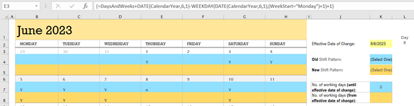
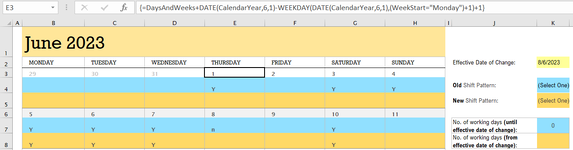
1) I redid the formula for calculating the calendar. Please look at the formula in cell B3.
2) I could not figure out what you meant by DaysAndWeeks, so I ignored that and used my guess at the formula in point 1.
3) Your calculations in cells L8 and L9 had a "double +", and you also reference cell L3 which is blank. You also have the same sign as the comparison operator in both formulas. So, I pretty much only used these formulas to get an idea of what you want. If my guess is wrong, please specify what you need.
4) I ignored your "day of month for consideration" (I'm guessing that is was L2 and L3 are for) in your calculations for L8 and L9. I just used the pure date value in cell K2.
5) The calculation I used in cells M7 and M8 are array formulas and work as a count if function. If you need to insert a calculation for the comparative values you can do that..... Just make sure you wrap that part in parentheses.
6) You can use the same kind of logic for calculations for K10 and K11. I just copied yours since they seemed to work.
7) The new formulas I've provided are K7,K8,K10,K11,B3,B6,B9,B12,B15
8) I do not have any idea what you want to do with the "drop down cells" in Cells K4 and K5.
9) I do no have any idea what you want to do with the "Y" values in rows: 8, 11,14,17
10) Not sure why you are "hard coding" the month name in you could make this formulaic pretty easily.

So, here is my xl2bb mini of your data:
I hope this helps:


Mr excel questions 39.xlsm
ABCDEFGHIJKLMNO
1June 2023DayCalendarYearWeekStartDaysAndWeeks
2MONDAYTUESDAYWEDNESDAYTHURSDAYFRIDAYSATURDAYSUNDAYEffective Date of Change:2023-06-0882023MONDAY
32930311234
4YYYOld Shift Pattern:(Select One)
5YYYNew Shift Pattern:(Select One)
6567891011
7YYYYNo. of working days (until effective date of change):6
8YYYYNo. of working days (from effective date of change):11
912131415161718
10YYYYNo. of working days in the month (assume full month roster):1717
11YYYNo. of working days in the month (assume full month roster):1616
1219202122232425
13YYY
14YYY
152627282930122023-05-29
16YYY
17YYY
kattay
Cell Formulas
RangeFormula
B1B1="June " & CalendarYear
B2:H2B2=UPPER(TEXT(B3,"dddd"))
B3B3=WORKDAY.INTL(DATE(2023,6,1)+1,-1,IF(WeekStart="MONDAY","0111111","1111110"))
C3:H3,C15:H15,C12:H12,C9:H9,C6:H6C3=B3+1
B6,B15,B12,B9B6=B3+7
M7M7=SUM((--(B4:H4="Y"))*(--(B3:H3)<K2))+ SUM((--(B7:H7="Y"))*(--(B6:H6)<K2))+ SUM((--(B10:H10="Y"))*(--(B9:H9)<K2))+ SUM((--(B13:H13="Y"))*(--(B12:H12)<K2))+ SUM((--(B16:H16="Y"))*(--(B15:H15)<K2))
M8M8=SUM((--(C4:I4="Y"))*(--(C3:I3)>=K2))+ SUM((--(C7:I7="Y"))*(--(C6:I6)>=K2))+ SUM((--(B10:H10="Y"))*(--(B9:H9)>=K2))+ SUM((--(B13:H13="Y"))*(--(B12:H12)>=K2))+ SUM((--(C16:I16="Y"))*(--(C15:I15)>=K2))
M10M10= COUNTIFS(B7:H7,"<>")+ COUNTIFS(B10:H10,"<>")+ COUNTIFS(B13:H13,"<>")+ COUNTIFS(B16:H16,"<>")+ COUNTIFS(B4:H4,"<>")
M11M11= COUNTIF(B8:H8,"<>")+ COUNTIF(B11:H11,"<>")+ COUNTIF(B14:H14,"<>")+ COUNTIF(B17:H17,"<>")+ COUNTIF(B5:H5,"<>")
J15J15=WORKDAY.INTL(DATE(2023,6,1)+1,-1,"0111111")
Named Ranges
NameRefers ToCells
CalendarYear=kattay!$M$2B1
WeekStart=kattay!$N$2B3
Cells with Data Validation
CellAllowCriteria
K4:K5List,Regular hours,2-rotating,3-rotating,Permanent night
 
Upvote 0

Forum statistics

Threads
1,215,069
Messages
6,122,954
Members
449,095
Latest member
nmaske

We've detected that you are using an adblocker.

We have a great community of people providing Excel help here, but the hosting costs are enormous. You can help keep this site running by allowing ads on MrExcel.com.
Allow Ads at MrExcel

Which adblocker are you using?

Disable AdBlock

Follow these easy steps to disable AdBlock

1)Click on the icon in the browser’s toolbar.
2)Click on the icon in the browser’s toolbar.
2)Click on the "Pause on this site" option.
Go back

Disable AdBlock Plus

Follow these easy steps to disable AdBlock Plus

1)Click on the icon in the browser’s toolbar.
2)Click on the toggle to disable it for "mrexcel.com".
Go back

Disable uBlock Origin

Follow these easy steps to disable uBlock Origin

1)Click on the icon in the browser’s toolbar.
2)Click on the "Power" button.
3)Click on the "Refresh" button.
Go back

Disable uBlock

Follow these easy steps to disable uBlock

1)Click on the icon in the browser’s toolbar.
2)Click on the "Power" button.
3)Click on the "Refresh" button.
Go back
Back
Top