Dates and conditional formatting

Tazzy666uk

New Member
Joined
Jul 15, 2014
Messages
19
Hi, I am getting in a bit of spin trying to sort this myself, and would like some help please.

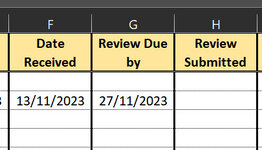
I have 3 columns I am referring to. Column G has a simple =F3+14 to give me 14 days on from the date in column F

However, what I would like (and my issue, which is stringing multiple formulas/conditional formatting together!!):


Assuming reference below to Row 3:

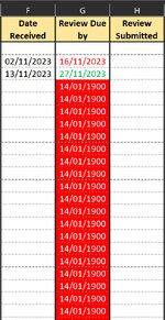
Text in G3 to be Green on days 1-4 of date in F3
Text in G3 to be orange on days 5-9 of date in F3
Text in G3 to be red on days 10-14 of date in F3
G3 cell to be filled red with white text when >14 days in F3

AND (sorry)

to not be conditional formatted at all once there is a date in Column H

If I cannot simply drag the formatting down the sheet, then this needs to apply to Rows 3-95

Hope that makes sense

Thank you so much in advance

Tazzy :)
 

Attachments

  • del excel.jpg
    del excel.jpg
    34.1 KB · Views: 11

Excel Facts

Excel motto
Not everything I do at work revolves around Excel. Only the fun parts.
Is this it?
Book1
FGH
1Date ReceivedReview Date byReview Submitted
2
331/10/202314/11/2023
41/11/202315/11/2023
52/11/202316/11/202314/11/2023
63/11/202317/11/2023
74/11/202318/11/2023
85/11/202319/11/202314/11/2023
96/11/202320/11/2023
107/11/202321/11/2023
118/11/202322/11/202314/11/2023
129/11/202323/11/2023
1310/11/202324/11/2023
1411/11/202325/11/2023
1512/11/202326/11/202314/11/2023
1613/11/202327/11/2023
1714/11/202328/11/2023
1815/11/202329/11/2023
1916/11/202330/11/2023
20
Sheet1
Cell Formulas
RangeFormula
G3:G19G3=F3+14
Cells with Conditional Formatting
CellConditionCell FormatStop If True
G3:G19Expression=AND(H3="",F3>=TODAY()-4,F3<TODAY()+1)textYES
G3:G19Expression=AND(H3="",F3>=TODAY()-9,F3<TODAY()+1)textYES
G3:G19Expression=AND(H3="",F3>=TODAY()-14,F3<TODAY()+1)textYES
G3:G19Expression=AND(H3="",F3<TODAY()-14)textYES
 
Upvote 0
You can have more than 3 rules now (not counting the default when none of the rules apply)?
 
Upvote 0
Is this it?
Book1
FGH
1Date ReceivedReview Date byReview Submitted
2
331/10/202314/11/2023
41/11/202315/11/2023
52/11/202316/11/202314/11/2023
63/11/202317/11/2023
74/11/202318/11/2023
85/11/202319/11/202314/11/2023
96/11/202320/11/2023
107/11/202321/11/2023
118/11/202322/11/202314/11/2023
129/11/202323/11/2023
1310/11/202324/11/2023
1411/11/202325/11/2023
1512/11/202326/11/202314/11/2023
1613/11/202327/11/2023
1714/11/202328/11/2023
1815/11/202329/11/2023
1916/11/202330/11/2023
20
Sheet1
Cell Formulas
RangeFormula
G3:G19G3=F3+14
Cells with Conditional Formatting
CellConditionCell FormatStop If True
G3:G19Expression=AND(H3="",F3>=TODAY()-4,F3<TODAY()+1)textYES
G3:G19Expression=AND(H3="",F3>=TODAY()-9,F3<TODAY()+1)textYES
G3:G19Expression=AND(H3="",F3>=TODAY()-14,F3<TODAY()+1)textYES
G3:G19Expression=AND(H3="",F3<TODAY()-14)textYES
Hi Kevin,

Firstly, Thank you for taking the time to do this for me, it is appreciated.

The formulas work, which is great, providing there is a date entered in Column F cells.... If it is blank, the cell is red with an odd date in..... I have tried entering the cell formula without the conditional formatting and I get the same date come up. Once I enter a date in cell F it all works as it should.

Ideally, I would like cells in column G to be clear and if there is no date in F...
 

Attachments

  • del excel 2.jpg
    del excel 2.jpg
    202.7 KB · Views: 2
Upvote 0
Could I suggest you make a slight change to your formula in column G, and a change to the last condition in the CF:
Book1
FGH
1Date ReceivedReview Date byReview Submitted
2
331/10/202314/11/2023
41/11/202315/11/2023
52/11/202316/11/202314/11/2023
6 
74/11/202318/11/2023
85/11/202319/11/202314/11/2023
96/11/202320/11/2023
10 
118/11/202322/11/202314/11/2023
129/11/202323/11/2023
1310/11/202324/11/2023
1411/11/202325/11/2023
1512/11/202326/11/202314/11/2023
1613/11/202327/11/2023
17 
1815/11/202329/11/2023
1916/11/202330/11/2023
20
Sheet1
Cell Formulas
RangeFormula
G3:G19G3=IF(ISNUMBER(F3),F3+14,"")
Cells with Conditional Formatting
CellConditionCell FormatStop If True
G3:G19Expression=AND(H3="",F3>=TODAY()-4,F3<TODAY()+1)textNO
G3:G19Expression=AND(H3="",F3>=TODAY()-9,F3<TODAY()+1)textNO
G3:G19Expression=AND(H3="",F3>=TODAY()-14,F3<TODAY()+1)textNO
G3:G19Expression=AND(H3="",ISNUMBER(F3),F3<TODAY()-14)textNO
 
Upvote 1
Solution
Could I suggest you make a slight change to your formula in column G, and a change to the last condition in the CF:
Book1
FGH
1Date ReceivedReview Date byReview Submitted
2
331/10/202314/11/2023
41/11/202315/11/2023
52/11/202316/11/202314/11/2023
6 
74/11/202318/11/2023
85/11/202319/11/202314/11/2023
96/11/202320/11/2023
10 
118/11/202322/11/202314/11/2023
129/11/202323/11/2023
1310/11/202324/11/2023
1411/11/202325/11/2023
1512/11/202326/11/202314/11/2023
1613/11/202327/11/2023
17 
1815/11/202329/11/2023
1916/11/202330/11/2023
20
Sheet1
Cell Formulas
RangeFormula
G3:G19G3=IF(ISNUMBER(F3),F3+14,"")
Cells with Conditional Formatting
CellConditionCell FormatStop If True
G3:G19Expression=AND(H3="",F3>=TODAY()-4,F3<TODAY()+1)textNO
G3:G19Expression=AND(H3="",F3>=TODAY()-9,F3<TODAY()+1)textNO
G3:G19Expression=AND(H3="",F3>=TODAY()-14,F3<TODAY()+1)textNO
G3:G19Expression=AND(H3="",ISNUMBER(F3),F3<TODAY()-14)textNO
Hi Kevin,

that is fantastic thank you. Added unintentional bonus that if I enter something in received with todays date or later, the cell font is black, not as per the conditional formatting, so I can populate the other cells in that row with what I ordered, and it now shows as black text to tell me it hasn't arrived yet..... perfect!

Really appreciate your help
 
Upvote 0

Forum statistics

Threads
1,215,069
Messages
6,122,959
Members
449,096
Latest member
Anshu121

We've detected that you are using an adblocker.

We have a great community of people providing Excel help here, but the hosting costs are enormous. You can help keep this site running by allowing ads on MrExcel.com.
Allow Ads at MrExcel

Which adblocker are you using?

Disable AdBlock

Follow these easy steps to disable AdBlock

1)Click on the icon in the browser’s toolbar.
2)Click on the icon in the browser’s toolbar.
2)Click on the "Pause on this site" option.
Go back

Disable AdBlock Plus

Follow these easy steps to disable AdBlock Plus

1)Click on the icon in the browser’s toolbar.
2)Click on the toggle to disable it for "mrexcel.com".
Go back

Disable uBlock Origin

Follow these easy steps to disable uBlock Origin

1)Click on the icon in the browser’s toolbar.
2)Click on the "Power" button.
3)Click on the "Refresh" button.
Go back

Disable uBlock

Follow these easy steps to disable uBlock

1)Click on the icon in the browser’s toolbar.
2)Click on the "Power" button.
3)Click on the "Refresh" button.
Go back
Back
Top