Extract Data from Single Cell. Column is Constant. Number of Rows Involved Changes. Number of Rows Within a Single Cell Can be 1 Up to 9

helpmeplz_

New Member
Joined
Aug 25, 2017
Messages
17
Office Version
  1. 365
Platform
  1. Windows
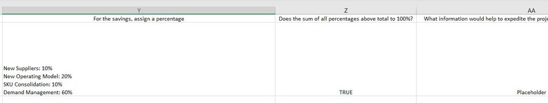
Hi, I am on a work computer so I can't download the plug to create a cool screenshot of data, but basically what I am trying to solve is that I download a file from a database that has a variable number of rows, but the columns are constant. I want to extract all data from column Y into up to 9 columns to the right of column AE (so beginning in column AF). The data in each row in column Y contains several rows within each cell (1-9 rows). This data looks like this:

RowColumn Y
1New Suppliers: 100%
2New Suppliers: 10%
New Operating Model: 10%
SKU Consolidation: 10%
Supplier Consolidation: 10%
Demand Management: 10%
Volume: 50%
3Strategic Negotiation: 10%
Sourcing Tool & Analytics: 50%
Commodity Market: 40%

The 9 columns with potential data (that would be extracted starting in column AF) would be named:

New Suppliers
New Operating Model
SKU Consolidation
Supplier Consolidation
Demand Management
Volume
Strategic Negotiation
Sourcing Tool & Analytics
Commodity Market

For each column, I would want to extract the corresponding percentage assigned to each in the same row (if applicable).
 

Attachments

  • Capture.JPG
    Capture.JPG
    34.2 KB · Views: 4

Excel Facts

Which Excel functions can ignore hidden rows?
The SUBTOTAL and AGGREGATE functions ignore hidden rows. AGGREGATE can also exclude error cells and more.
How about this?
Book1
YAFAGAHAIAJAKALAMAN
1New SuppliersNew Operating ModelSKU ConsolidationSupplier ConsolidationDemand ManagementVolumeStrategic NegotiationSourcing Tool & AnalyticsCommodity Market
2New Suppliers: 100% 100%
3New Suppliers: 10% New Operating Model: 10% SKU Consolidation: 10% Supplier Consolidation: 10% Demand Management: 10% Volume: 50% 10% 10% 10% 10% 10% 50%
4Strategic Negotiation: 10% Sourcing Tool & Analytics: 50% Commodity Market: 40%  10% 50% 40%
Sheet7
Cell Formulas
RangeFormula
AF2:AN4AF2=LET( a,XMATCH(TEXTBEFORE(TEXTSPLIT(Y2,CHAR(10)),":"),$AF$1:$AO$1), b,TEXTAFTER(TEXTSPLIT(Y2,CHAR(10)),":"), XLOOKUP(SEQUENCE(1,9),a,b,""))
Dynamic array formulas.
 
Upvote 0
Here also a Power Query solution.

Power Query:
let
    Source = Excel.CurrentWorkbook(){[Name="Table1"]}[Content],
    cols = {"New Suppliers", "New Operating Model", "SKU Consolidation", "Supplier Consolidation", "Demand Management", "Volume", "Strategic Negotiation", "Sourcing Tool & Analytics", "Commodity Market"},
    nCol = Table.AddColumn(Source, "Custom", each
             let 
                tbl = Table.FromRows(List.Transform(Text.Split([Info],"#(lf)"), (x)=> Text.Split(x,": "))),
                colNames = List.Select(cols, (x)=> List.PositionOf(tbl[Column1],x)>=0),
                tblNew = Table.ReorderColumns(Table.PromoteHeaders(Table.Transpose(tbl)),colNames)
             in
                tblNew      
        ),
    result = Table.ExpandTableColumn(nCol, "Custom", cols, cols)
in
    result

Book1
ABCDEFGHIJK
1NrInfo
21New Suppliers: 100%
32New Suppliers: 10% New Operating Model: 10% SKU Consolidation: 10% Supplier Consolidation: 10% Demand Management: 10% Volume: 50%
43Strategic Negotiation: 10% Sourcing Tool & Analytics: 50% Commodity Market: 40%
5
6
7
8
9
10NrInfoNew SuppliersNew Operating ModelSKU ConsolidationSupplier ConsolidationDemand ManagementVolumeStrategic NegotiationSourcing Tool & AnalyticsCommodity Market
111New Suppliers: 100%100%
122New Suppliers: 10% New Operating Model: 10% SKU Consolidation: 10% Supplier Consolidation: 10% Demand Management: 10% Volume: 50%10%10%10%10%10%50%
133Strategic Negotiation: 10% Sourcing Tool & Analytics: 50% Commodity Market: 40%10%50%40%
Sheet1
 
Upvote 0
How about this?
Book1
YAFAGAHAIAJAKALAMAN
1New SuppliersNew Operating ModelSKU ConsolidationSupplier ConsolidationDemand ManagementVolumeStrategic NegotiationSourcing Tool & AnalyticsCommodity Market
2New Suppliers: 100% 100%
3New Suppliers: 10% New Operating Model: 10% SKU Consolidation: 10% Supplier Consolidation: 10% Demand Management: 10% Volume: 50% 10% 10% 10% 10% 10% 50%
4Strategic Negotiation: 10% Sourcing Tool & Analytics: 50% Commodity Market: 40%  10% 50% 40%
Sheet7
Cell Formulas
RangeFormula
AF2:AN4AF2=LET( a,XMATCH(TEXTBEFORE(TEXTSPLIT(Y2,CHAR(10)),":"),$AF$1:$AO$1), b,TEXTAFTER(TEXTSPLIT(Y2,CHAR(10)),":"), XLOOKUP(SEQUENCE(1,9),a,b,""))
Dynamic array formulas.
This works, but the data comes out as either text or something else. It can't be summed to ensure it's 100% total. Pivot table doesn't recognize it as a number either.
 
Upvote 0
This will return as decimal. You can format the cells as % if needed.

Excel Formula:
=LET(
a,XMATCH(TEXTBEFORE(TEXTSPLIT(Y2,CHAR(10)),":"),$AF$1:$AO$1),
b,TEXTAFTER(TEXTSPLIT(Y2,CHAR(10)),":"),
XLOOKUP(SEQUENCE(1,9),a,NUMBERVALUE(TRIM(b)),""))
 
Upvote 0
This will return as decimal. You can format the cells as % if needed.

Excel Formula:
=LET(
a,XMATCH(TEXTBEFORE(TEXTSPLIT(Y2,CHAR(10)),":"),$AF$1:$AO$1),
b,TEXTAFTER(TEXTSPLIT(Y2,CHAR(10)),":"),
XLOOKUP(SEQUENCE(1,9),a,NUMBERVALUE(TRIM(b)),""))
That's it, worked perfectly! Thank you!
 
Upvote 0

Forum statistics

Threads
1,215,219
Messages
6,123,688
Members
449,117
Latest member
Aaagu

We've detected that you are using an adblocker.

We have a great community of people providing Excel help here, but the hosting costs are enormous. You can help keep this site running by allowing ads on MrExcel.com.
Allow Ads at MrExcel

Which adblocker are you using?

Disable AdBlock

Follow these easy steps to disable AdBlock

1)Click on the icon in the browser’s toolbar.
2)Click on the icon in the browser’s toolbar.
2)Click on the "Pause on this site" option.
Go back

Disable AdBlock Plus

Follow these easy steps to disable AdBlock Plus

1)Click on the icon in the browser’s toolbar.
2)Click on the toggle to disable it for "mrexcel.com".
Go back

Disable uBlock Origin

Follow these easy steps to disable uBlock Origin

1)Click on the icon in the browser’s toolbar.
2)Click on the "Power" button.
3)Click on the "Refresh" button.
Go back

Disable uBlock

Follow these easy steps to disable uBlock

1)Click on the icon in the browser’s toolbar.
2)Click on the "Power" button.
3)Click on the "Refresh" button.
Go back
Back
Top