extract values based on next two columns

noubaba

New Member
Joined
Apr 10, 2018
Messages
19
Dear Experts,
Need your help to develop a formula,
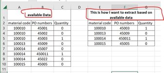
I have some data in "available Data" table and in other excel sheet I have some material codes in column E, which I want to lookup but the condition is for example if this code 100010 having zero in column C then it must be skipped and return valve must be 45003 and in F3 and 1 in G3, and if any code like 100013 do not have 1 in column C then return value must be 45009 in F4 and 0 in G4. Moreover For code 100015 there are two PO numbers 45005 and 450020 and both having zero in column C, in this case latest value with 450020 must be captured in F6. attached picture can be referred as well. Thank you

question Book1.xlsx
ABCDEFG
1available DataThis is how I want to extract based on available data
2material codePO numbers Quantitymaterial codePO numbers Quantity
3100010450010100010450031
4100010450020100013450090
51000104500311000144500111
61000134500901000154500200
7100014450070
81000144500111
9100014450220
10100015450050
111000154500200
Sheet1
 

Attachments

  • Excel post for help.JPG
    Excel post for help.JPG
    81.3 KB · Views: 1

Excel Facts

Test for Multiple Conditions in IF?
Use AND(test, test, test, test) or OR(test, test, test, ...) as the logical_test argument of IF.
You have not told us what your Excel product is... If it is O365, try this:

It assumes that your first row of DATA is in cell A3, and that the area where you expect results to appear is BLANK.

=LET(A,A3:A11,B,B3:C11,C,UNIQUE(A),VSTACK(A2:C2,HSTACK(C,DROP(REDUCE("",C,LAMBDA(x,y,(VSTACK(x,IFERROR(FILTER(B,(A=y)*(INDEX(B,,2)<>0)),TAKE(FILTER(B,A=y),-1)))))),1))))
 
Upvote 0
Book1.xlsx
ABCDEFG
1
2material codePO numbersQuantitymaterial codePO numbersQuantity
3100010450010100010450031
4100010450020100013450090
51000104500311000144500111
61000134500901000154500200
7100014450070
81000144500111
9100014450220
10100015450050
111000154500200
12
Sheet1
Cell Formulas
RangeFormula
E2:G6E2=LET(A,A3:A11,B,B3:C11,C,UNIQUE(A),VSTACK(A2:C2,HSTACK(C,DROP(REDUCE("",C,LAMBDA(x,y,(VSTACK(x,IFERROR(FILTER(B,(A=y)*(INDEX(B,,2)<>0)),TAKE(FILTER(B,A=y),-1)))))),1))))
Dynamic array formulas.
 
Upvote 0
I have office pro plus 2016,
Thank You Glenn for your help but this is not what I want, please allow me to explain again.
I have table 1 in one sheet and on the other sheet I have table 2. In table 2 I have only material codes in column E which I want to look up in table 1 range. But I want to capture specific PO numbers in column F and Quantity in G. for example as I mentioned in table 3. I need Vlookup or Xlookup or any other formula which I can apply in F3 and G3 and then drag below.

question Book1.xlsx
ABCDEFGHIJK
1table 1Table 2Table 3 - Result after lookup material codes in table 1. Want to capture specific PO numbers and Quantity
2material codePO numbers Quantitymaterial codePO numbers Quantitymaterial codePO numbers Quantity
3100010450010100010100010450031
4100010450020100013100013450090
51000104500311000141000144500111
61000134500901000151000154500200
7100014450070
81000144500111
9100014450220
10100015450050
111000154500200
Sheet1 (2)
 
Upvote 0
Your explanation is FAR from clear. Obviously my first attempt won't work with your older Excel product. So try this (again a guess, as your requirement was not at all clear):

Book4.xlsx
ABCDEFGHI
1
22material codePO numbersQuantitymaterial codePO numbersQuantity
33100010450010100010450031
44100010450020100013450090
551000104500311000144500111
661000134500901000154500200
77100014450070  
881000144500111  
99100014450220  
1010100015450050  
11111000154500200
12
13
14
15
Sheet1
Cell Formulas
RangeFormula
G3:H10G3=IF($F3="","",INDEX(C:C,AGGREGATE(14,6,ROW($B$3:$B$19)/(($B$3:$B$19=$F3)*(IF(SUMIF($B:$B,$F3,$D:$D)=0,1,($D$3:$D$19<>0)))),1)))
 
Upvote 0
In the above... the formula returns the row corresponding to the last non-zero value in columns C for each code. If all values in column C, for an individual code, are zero, it returns the last one.
 
Upvote 0
In your sample data, it appears that if there is a 1, it is your highest # PO. If that is actually the case then I think this should work.

Book2
ABCDEFG
1material codePO numbersQuantitymaterial codePO numbersQuantity
2100010450010100010450031
3100010450020100013450090
41000104500311000144500111
51000134500901000154500200
6100014450070
71000144500111
8100014450220
9100015450050
101000154500200
Sheet1
Cell Formulas
RangeFormula
F2:G5F2=MAXIFS(B:B,$A:$A,$E2)
 
Upvote 0
I have office pro plus 2016,

I suggest that you update your Account details (or click your user name at the top right of the forum) so helpers always know what Excel version(s) & platform(s) you are using as the best solution often varies by version. (Don’t forget to scroll down & ‘Save’)
 
Upvote 0

Forum statistics

Threads
1,215,350
Messages
6,124,431
Members
449,158
Latest member
burk0007

We've detected that you are using an adblocker.

We have a great community of people providing Excel help here, but the hosting costs are enormous. You can help keep this site running by allowing ads on MrExcel.com.
Allow Ads at MrExcel

Which adblocker are you using?

Disable AdBlock

Follow these easy steps to disable AdBlock

1)Click on the icon in the browser’s toolbar.
2)Click on the icon in the browser’s toolbar.
2)Click on the "Pause on this site" option.
Go back

Disable AdBlock Plus

Follow these easy steps to disable AdBlock Plus

1)Click on the icon in the browser’s toolbar.
2)Click on the toggle to disable it for "mrexcel.com".
Go back

Disable uBlock Origin

Follow these easy steps to disable uBlock Origin

1)Click on the icon in the browser’s toolbar.
2)Click on the "Power" button.
3)Click on the "Refresh" button.
Go back

Disable uBlock

Follow these easy steps to disable uBlock

1)Click on the icon in the browser’s toolbar.
2)Click on the "Power" button.
3)Click on the "Refresh" button.
Go back
Back
Top