Filtered Named Range display questions

[jdt102010]

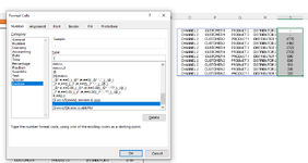
1. The highlighted formula (YELLOW) is filtering a named range from another sheet, and displaying only the first five columns. Notice that the Target Date column is 1/0/1900 (RED) This is because there is no date entered in that cell in the named range. How do I write the formula to display a blank cell (or something like "NA") in these cases?
2. The Task name in column B (BLUE) isn't showing all of the task name, because it isn't wrapping the text. Is it possible to make it so it will always wrap the text for this column?
3. Finally, is there a way to put two of these filtered named ranges on the same page one over the other (vertically), so that depending on the number of rows, it bumps down the lower table to accommodate larger numbers of rows?

 

[RICH937]

So I spent some time on this, and you're right. It's weird. I was sure that simply typing "" in the if_empty field would produce a blank space. Particularly since the vid on the link below says to do exactly that at the 49 second mark. Doesn't work though. The dynamic array I built to troubleshoot this always returns with zeros. I did find a workaround, but it's far from ideal. You can go into format cells-->number, and select "custom" in the type field you can type anything you'd like and that is what will be displayed for zeros. In the example I have pictured, I chose a single dash. The issue is, when you do enter in the dates, you'll have to go back in and change the format to date. Best I can do bro.

FILTER function - Microsoft Support

How to use the FILTER function in Excel to filter a range of data based on criteria you define.

support.microsoft.com

 

[Fluff]

Can you post both formulae, rather than an image of one of them.

 

[jdt102010]

Here is the formula: =CHOOSECOLS(FILTER(tasklist,tasklist[Client]=A1),1,2,3,4,5)

 

[Fluff]

And the other formula you want to stack below it?

 

[BrettJH]

You can change the Number formatting in Custom Number Formats to show dates when there is a date and either nothing or any text string in place of zero values by adding 2 semicolons after the date format to define the zero number format.

to display as nothing add 2 semicolons after the custom number format:
mm/dd/yyyy;;

to add "N/A" in place of zeros
mm/dd/yyyy;;"N/A"

 

[jdt102010]

The named range is "tasklist" and the column name is "Client". This formula compares

And the other formula you want to stack below it?

It would be essentially the same formula with an additional criteria that filters another column in the same named range. These are tasks, and they have a column that indicates status. As the status changes, that task be picked up by these filters accordingly. Does that make sense?

 

[Fluff]

Try like

=let(a,CHOOSECOLS(FILTER(tasklist,tasklist[Client]=A1),1,2,3,4,5),b,your other formula,VSTACK(IF(a="","",a),IF(b="","",b)))