Vincent88
Active Member
- Joined
- Mar 5, 2021
- Messages
- 382
- Office Version
- 2019
- Platform
- Windows
- Mobile
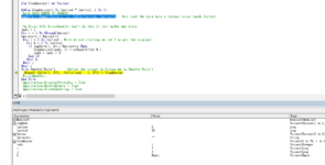
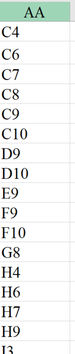
Hi Guys, I want to find the cell addresses to a Arraylist (blankarray) of those values in an array (bArray). It seems that the code adds those blank cells' addresses only but not those values to Arraylist. Please advise correction to my code to make it works.
Also I want to list those findings of each row in individual column in the Arraylist (meaning findings of row 3 in rngData shown in column 1 of Arraylist , that of row 4 shown in column 2 of Arraylist and so on).
Thanks.
Also I want to list those findings of each row in individual column in the Arraylist (meaning findings of row 3 in rngData shown in column 1 of Arraylist , that of row 4 shown in column 2 of Arraylist and so on).
Thanks.
VBA Code:
Sub rngOver32()

Dim cl As Range, rngData As Range

Application.DisplayStatusBar = False
Application.EnableEvents = False
Application.ScreenUpdating = False


Dim lastrow As Long, lastcol As Long
lastrow = Range("A3").End(xlDown).Row
lastcol = Cells(1, Columns.Count).End(xlToLeft).Column

'LIST OF VALUE TO FIND
Dim bArray As Variant
bArray = Array("AL", "SL", "BL", "CL", "PL", "VL", vbNullString)
Dim bArraystr As String


'EXPORT CELL ADDRESSES TO ARRAYLIST
Dim blankarray As Object
Set blankarray = CreateObject("System.Collections.ArrayList")

'SET DATA RANGE TO SEARCH
Set rngData = Range(Cells(3, 3), Cells(lastrow, lastcol))
Debug.Print rngData.Address

On Error GoTo ErrorHandler

For Each cl In rngData
    If cl.Value = bArraystr Then
       If Not blankarray.contains(cl.Address) Then blankarray.Add cl.Address
    End If
Next cl

ErrorHandler:
Application.EnableEvents = True

Application.DisplayStatusBar = True
Application.EnableEvents = True
Application.ScreenUpdating = True

End Sub| AgentProposal_Roster0728_1025M.xlsm | ||||||||||||||||||||||||||||||||||||||||
|---|---|---|---|---|---|---|---|---|---|---|---|---|---|---|---|---|---|---|---|---|---|---|---|---|---|---|---|---|---|---|---|---|---|---|---|---|---|---|---|---|
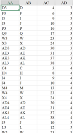
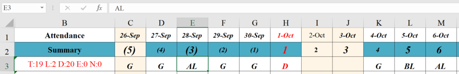
| A | B | C | D | E | F | G | H | I | J | K | L | M | N | O | P | Q | R | S | T | U | V | W | X | Y | Z | AA | AB | AC | AD | AE | AF | AG | AH | AI | AJ | AK | AL | |||
| 1 | MDate | Attendance | 26-Nov | 27-Nov | 28-Nov | 29-Nov | 30-Nov | 1-Dec | 2-Dec | 3-Dec | 4-Dec | 5-Dec | 6-Dec | 7-Dec | 8-Dec | 9-Dec | 10-Dec | 11-Dec | 12-Dec | 13-Dec | 14-Dec | 15-Dec | 16-Dec | 17-Dec | 18-Dec | 19-Dec | 20-Dec | 21-Dec | 22-Dec | 23-Dec | 24-Dec | 25-Dec | 26-Dec | 27-Dec | 28-Dec | 29-Dec | 30-Dec | 31-Dec | ||
| 2 | Date | Summary | (5) | (4) | (3) | (2) | (1) | 1 | 2 | 3 | 4 | 5 | 6 | 7 | 8 | 9 | 10 | 11 | 12 | 13 | 14 | 15 | 16 | 17 | 18 | 19 | 20 | 21 | 22 | 23 | 24 | 25 | 26 | 27 | 28 | 29 | 30 | 31 | ||
| 3 | Xia M | T:22 L:2.5 D:16.5 E:7 N:0 | G | G | G | G | G | G | VL | VL | G | G | D | K | E | E | E | D | D | D | D | D | AM | D | D | D | D | D | D | E | E | E | E | |||||||
| 4 | Zita V | T:22 L:1 D:12 E:11 N:0 | D | D | D | D | D | D | D | E | E | E | E | E | D | D | D | D | D | D | D | D | CL | E | E | E | E | E | E | |||||||||||
| 5 | Ken C | T:22 L:6 D:5 E:5 N:11 | K | K | K | K | K | K | K | K | AL | N | N | N | N | N | E | E | E | E | E | AL | N | N | N | N | N | N | AL | AL | AL | AL | ||||||||
| 6 | Larry Q | T:22 L:0 D:15 E:0 N:0 | D3 | D3 | D3 | D3 | D3 | D3 | D3 | D4 | D4 | D4 | D4 | D4 | D4 | D4 | D4 | D4 | D4 | G | ||||||||||||||||||||
| 7 | John G | T:22 L:0.5 D:17.5 E:5 N:0 | E | E | E | E | E | E | E | D1 | D1 | D1 | G | G | G | G | G | PM | G | G | G | G | G | G | G | G | G | |||||||||||||
202112 | ||||||||||||||||||||||||||||||||||||||||
| Cells with Data Validation | ||
|---|---|---|
| Cell | Allow | Criteria |
| A3:A7 | List | =HelpAgent |
| H3:AL7 | List | =ShiftcodeNew |
| A1 | List | =Data!$U$2:$U$15 |