Finding a number 10 less than the highest rating number, in a specific date and time range.

[Moggsy85]

Hi

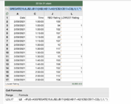
A user kindly provided me with the formula in the image below (=IF(J3=AGGREGATE(15,6,J$2:J$17/((A$2:A$17=A3)*(C$2:C$17=C3)),1),1,""), which highlights the lowest rating in a specific time and date.

However, I am now looking to see if i can add something to it. I want to find the lowest rating within the time and date, but i would like the rating to be a minimum of 10 less than the highest rating?

So for example in the image where L14 was selected as it was the lowest of the 3 ratings, I would like that to have NOT been highlighted as it is not a minimum of 10 less than the highest rating in that time and date.

Many thanks

 

[KRice]

Try this...looks like this is an extension from thread:

Finding lowest value in time and date

Hi, is it possible to add a formula to the LOWEST rating cell to highlight the lowest RBD rating, based on the date and specific time? Many thanks Date Track Time Horse Industry SP Betfair SP IP Min IP Max Place RBD Rating RBD Rank LOWEST Rating 02/09/2021 SALISBURY 01:00:00 Rectory Road...

www.mrexcel.com

...which is where I obtained the source table and Peter's initial formula for the Lowest Rating.

Book1
	A		C							J		L	M
1	Date		Time							RBD Rating		LOWEST Rating	Lowest AND min of 10 less than MAX
2	2-Sep-21		1:00:00							109
3	2-Sep-21		1:00:00							94		1	1
4	2-Sep-21		1:00:00							102
5	2-Sep-21		1:15:00							157
6	2-Sep-21		1:15:00							20		1	1
7	2-Sep-21		1:15:00							107
8	2-Sep-21		1:30:00							10		1	1
9	2-Sep-21		1:30:00							117
10	2-Sep-21		1:30:00							105
11	2-Sep-21		1:30:00							10		1	1
12	2-Sep-21		1:45:00							153
13	2-Sep-21		1:45:00							158
14	2-Sep-21		1:45:00							152		1
15	2-Sep-21		2:00:00							102		1	1
16	2-Sep-21		2:00:00							112
17	2-Sep-21		2:00:00							104
Sheet1

Cell Formulas
Range	Formula
L2:L17	L2	=IF(J2=AGGREGATE(15,6,J$2:J$17/((A$2:A$17=A2)*(C$2:C$17=C2)),1),1,"")
M2:M17	M2	=IF(AND(J2=AGGREGATE(15,6,$J$2:$J$17/(($A$2:$A$17=$A2)*($C$2:$C$17=$C2)),1),J2<=AGGREGATE(14,6,$J$2:$J$17/(($A$2:$A$17=$A2)*($C$2:$C$17=$C2)),1)-10),1,"")

 

[Moggsy85]

Try this...looks like this is an extension from thread:

Finding lowest value in time and date

Hi, is it possible to add a formula to the LOWEST rating cell to highlight the lowest RBD rating, based on the date and specific time? Many thanks Date Track Time Horse Industry SP Betfair SP IP Min IP Max Place RBD Rating RBD Rank LOWEST Rating 02/09/2021 SALISBURY 01:00:00 Rectory Road...

www.mrexcel.com

...which is where I obtained the source table and Peter's initial formula for the Lowest Rating.

Book1
	A		C							J		L	M
1	Date		Time							RBD Rating		LOWEST Rating	Lowest AND min of 10 less than MAX
2	2-Sep-21		1:00:00							109
3	2-Sep-21		1:00:00							94		1	1
4	2-Sep-21		1:00:00							102
5	2-Sep-21		1:15:00							157
6	2-Sep-21		1:15:00							20		1	1
7	2-Sep-21		1:15:00							107
8	2-Sep-21		1:30:00							10		1	1
9	2-Sep-21		1:30:00							117
10	2-Sep-21		1:30:00							105
11	2-Sep-21		1:30:00							10		1	1
12	2-Sep-21		1:45:00							153
13	2-Sep-21		1:45:00							158
14	2-Sep-21		1:45:00							152		1
15	2-Sep-21		2:00:00							102		1	1
16	2-Sep-21		2:00:00							112
17	2-Sep-21		2:00:00							104
Sheet1

Cell Formulas
Range	Formula
L2:L17	L2	=IF(J2=AGGREGATE(15,6,J$2:J$17/((A$2:A$17=A2)*(C$2:C$17=C2)),1),1,"")
M2:M17	M2	=IF(AND(J2=AGGREGATE(15,6,$J$2:$J$17/(($A$2:$A$17=$A2)*($C$2:$C$17=$C2)),1),J2<=AGGREGATE(14,6,$J$2:$J$17/(($A$2:$A$17=$A2)*($C$2:$C$17=$C2)),1)-10),1,"")

Hi, the formula works perfectly, but lets say I add a filter that takes out any rating under 100, when i add the formula it still calculates those ratings i filtered out? IS there a way around this?

 

[KRice]

That's a different matter. Most functions will use all values in a specified range, but there are some that will operate only on visible cells after an autofilter is applied (e.g., SUBTOTAL). One approach is to build the capacity for a filter directly into the formula, as shown in the yellow filter input cells and column N.

MrExcel_20220424.xlsx
	A		C							J		L	M	N
1													use vals >=	100
2	Date		Time							RBD Rating		LOWEST Rating	Lowest AND min of 10 less than MAX	Lowest AND min of 10 less than MAX on filtering ratings
3	2-Sep-21		1:00:00							109
4	2-Sep-21		1:00:00							94		1	1
5	2-Sep-21		1:00:00							102
6	2-Sep-21		1:15:00							157
7	2-Sep-21		1:15:00							20		1	1
8	2-Sep-21		1:15:00							107				1
9	2-Sep-21		1:30:00							10		1	1
10	2-Sep-21		1:30:00							117
11	2-Sep-21		1:30:00							105				1
12	2-Sep-21		1:30:00							10		1	1
13	2-Sep-21		1:45:00							153
14	2-Sep-21		1:45:00							158
15	2-Sep-21		1:45:00							152		1
16	2-Sep-21		2:00:00							102		1	1	1
17	2-Sep-21		2:00:00							112
18	2-Sep-21		2:00:00							104
Sheet1

Cell Formulas
Range	Formula
L3:L18	L3	=IF(J3=AGGREGATE(15,6,J$3:J$18/((A$3:A$18=A3)*(C$3:C$18=C3)),1),1,"")
M3:M18	M3	=IF(AND(J3=AGGREGATE(15,6,$J$3:$J$18/(($A$3:$A$18=$A3)*($C$3:$C$18=$C3)),1),J3<=AGGREGATE(14,6,$J$3:$J$18/(($A$3:$A$18=$A3)*($C$3:$C$18=$C3)),1)-10),1,"")
N3:N18	N3	=IF(AND(J3=AGGREGATE(15,6,$J$3:$J$18/(($A$3:$A$18=$A3)*($C$3:$C$18=$C3)*($J$3:$J$18>=$N$1)),1),J3<=AGGREGATE(14,6,$J$3:$J$18/(($A$3:$A$18=$A3)*($C$3:$C$18=$C3)*($J$3:$J$18>=$N$1)),1)-10),1,"")

 

[Moggsy85]

That's a different matter. Most functions will use all values in a specified range, but there are some that will operate only on visible cells after an autofilter is applied (e.g., SUBTOTAL). One approach is to build the capacity for a filter directly into the formula, as shown in the yellow filter input cells and column N.

MrExcel_20220424.xlsx
	A		C							J		L	M	N
1													use vals >=	100
2	Date		Time							RBD Rating		LOWEST Rating	Lowest AND min of 10 less than MAX	Lowest AND min of 10 less than MAX on filtering ratings
3	2-Sep-21		1:00:00							109
4	2-Sep-21		1:00:00							94		1	1
5	2-Sep-21		1:00:00							102
6	2-Sep-21		1:15:00							157
7	2-Sep-21		1:15:00							20		1	1
8	2-Sep-21		1:15:00							107				1
9	2-Sep-21		1:30:00							10		1	1
10	2-Sep-21		1:30:00							117
11	2-Sep-21		1:30:00							105				1
12	2-Sep-21		1:30:00							10		1	1
13	2-Sep-21		1:45:00							153
14	2-Sep-21		1:45:00							158
15	2-Sep-21		1:45:00							152		1
16	2-Sep-21		2:00:00							102		1	1	1
17	2-Sep-21		2:00:00							112
18	2-Sep-21		2:00:00							104
Sheet1

Cell Formulas
Range	Formula
L3:L18	L3	=IF(J3=AGGREGATE(15,6,J$3:J$18/((A$3:A$18=A3)*(C$3:C$18=C3)),1),1,"")
M3:M18	M3	=IF(AND(J3=AGGREGATE(15,6,$J$3:$J$18/(($A$3:$A$18=$A3)*($C$3:$C$18=$C3)),1),J3<=AGGREGATE(14,6,$J$3:$J$18/(($A$3:$A$18=$A3)*($C$3:$C$18=$C3)),1)-10),1,"")
N3:N18	N3	=IF(AND(J3=AGGREGATE(15,6,$J$3:$J$18/(($A$3:$A$18=$A3)*($C$3:$C$18=$C3)*($J$3:$J$18>=$N$1)),1),J3<=AGGREGATE(14,6,$J$3:$J$18/(($A$3:$A$18=$A3)*($C$3:$C$18=$C3)*($J$3:$J$18>=$N$1)),1)-10),1,"")

THank you so much, And just out of interest, if i was to look for the highest rating instead of the lowest, how would i adapt this formula?
=IF(AQ2=AGGREGATE(15,6,AQ$2:AQ$111000/((A$2:A$111000=A2)*(H$2:H$111000=h2)),1),1,"")

 

[KRice]

Changing the 15 to a 14...as in AGGREGATE(14...will return the largest value in the array found in the 3rd argument of the AGGREGATE function.

 

[Moggsy85]

Changing the 15 to a 14...as in AGGREGATE(14...will return the largest value in the array found in the 3rd argument of the AGGREGATE function.

Thank you