Formulas Not Auto Filling

mparker173499

New Member
Joined
Mar 20, 2024
Messages
2
Office Version
  1. 365
Platform
  1. Windows
I have a sales table with several columns containing formulas. Daily we refresh the data to bring in the sales from the previous day. Problem is the formulas don't populate into the new rows created by the new sales. Heres what you should know...

It is a table

I read someplace the formula needs to be created next to the data when it is a table. This solved the problem on the first refresh but formulas didn't populate on the next refresh

I tried to band-aid it by using a macro to autofill the formulas from the first row down but there is so much data it takes forever.

It is a multiple user office setting so it is not realistic for everyone to refresh and manually fill the formulas each time they use it
 

Excel Facts

How to show all formulas in Excel?
Press Ctrl+` to show all formulas. Press it again to toggle back to numbers. The grave accent is often under the tilde on US keyboards.
Hey MP,
Hard to help without actually being able to see what you're working with. If you can, download the XL2BB add-in. it's a little quirky when you start, but after using a few times, it's great. I usually turn it off whenever I'm not actively using for this board.

Just in case you cannot, I went ahead and pulled a simple YTD sales table that is fed from daily sales and compares YTD performance with an annual sales Plan.

The blue table is what I built to represent daily sales and total sales prior to 3/17/2024. I built it with 4 days of random sales. Use the select date dropdown to pick a day, and watch what the results table does.

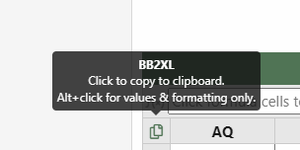
Reading your initial comments, I think this is what you're trying to do? click on the icon in the pic at the top of the tables here on the board, and it will let you paste both tables directly into excel. We can discuss what you're needing easier after that.

Let me know also about the size of the tables you're working with. My daily sales tables and annual roll ups are usually in the 25K-30K line range. Are you about the same?

new attempt at pareto source2.xlsb
ABCDEFGHIJKLMNOP
1FEEDER TABLE5152535455262RESULTS TABLESELECT DATE èèè3/18/2024
2PRODUCTYTD START3/18/20243/19/20243/20/20243/21/2024YTD SALES ( SEL. DATE)PRODUCTYTD 2024 VS 20232023 YTD SALES2024 YTD SALESYTD PLAN2024 PLAN TOTALACT V PLAN YTD% YTD PLAN
3PRODUCT 1$638,596$12,162$10,488$12,151$12,139$650,758PRODUCT 1-29.0%$916,508$650,758$594,048$2,993,088$56,7109.5%
4PRODUCT 2$892,770$16,748$14,870$17,267$15,771$909,518PRODUCT 2-11.1%$1,023,292$909,518$851,916$4,292,346$57,6026.8%
5PRODUCT 3$352,332$7,417$6,692$6,641$7,318$359,749PRODUCT 322.6%$293,314$359,749$377,260$1,900,810-$17,511-4.6%
6PRODUCT 4$249,404$4,577$4,390$4,226$4,636$253,981PRODUCT 422.6%$207,155$253,981$235,248$1,185,288$18,7338.0%
7PRODUCT 5$822,155$18,147$16,037$15,328$18,170$840,302PRODUCT 5753.3%$98,477$840,302$867,256$4,369,636-$26,954-3.1%
8PRODUCT 6$736,672$15,229$15,839$13,611$13,820$751,901PRODUCT 61584.7%$44,631$751,901$778,596$3,922,926-$26,695-3.4%
9PRODUCT 7$132,737$2,604$2,273$2,269$2,470$135,341PRODUCT 7-18.2%$165,419$135,341$124,800$628,800$10,5418.4%
10PRODUCT 8$374,719$7,607$6,401$6,851$6,444$382,326PRODUCT 84759.3%$7,868$382,326$360,048$1,814,088$22,2786.2%
11PRODUCT 9$837,562$16,790$14,663$17,410$15,335$854,352PRODUCT 923.1%$693,912$854,352$824,408$4,153,748$29,9443.6%
12PRODUCT 10$865,301$16,714$15,262$14,603$16,231$882,015PRODUCT 101577.9%$52,567$882,015$838,812$4,226,322$43,2035.2%
13PRODUCT 11$519,310$10,547$10,305$12,138$11,377$529,857PRODUCT 11183.4%$186,936$529,857$588,172$2,963,482-$58,315-9.9%
14PRODUCT 12$832,514$17,913$16,796$17,896$19,110$850,427PRODUCT 121063.7%$73,078$850,427$911,196$4,591,026-$60,769-6.7%
15PRODUCT 13$356,557$6,715$7,701$7,545$7,449$363,272PRODUCT 133551.0%$9,950$363,272$369,772$1,863,082-$6,500-1.8%
16PRODUCT 14$600,948$9,943$10,317$10,639$11,350$610,891PRODUCT 142041.4%$28,527$610,891$562,120$2,832,220$48,7718.7%
17PRODUCT 15$96,856$2,046$1,911$2,035$2,080$98,902PRODUCT 1575.9%$56,235$98,902$104,000$524,000-$5,098-4.9%
18PRODUCT 16$682,764$14,001$13,480$14,439$14,309$696,765PRODUCT 162569.1%$26,105$696,765$703,664$3,545,384-$6,899-1.0%
19PRODUCT 17$679,694$13,335$12,151$11,783$12,507$693,029PRODUCT 172174.5%$30,469$693,029$661,076$3,330,806$31,9534.8%
20PRODUCT 18$107,086$1,820$2,069$2,060$1,749$108,906PRODUCT 18341.5%$24,668$108,906$100,828$508,018$8,0788.0%
21PRODUCT 19$883,023$15,059$17,113$15,158$17,172$898,082PRODUCT 195980.4%$14,770$898,082$855,504$4,310,424$42,5785.0%
22PRODUCT 20$1,028,721$20,623$20,700$17,955$20,393$1,049,344PRODUCT 203650.6%$27,978$1,049,344$1,006,876$5,073,106$42,4684.2%
23PRODUCT 21$357,374$6,800$6,202$5,965$6,738$364,174PRODUCT 213788.3%$9,366$364,174$337,116$1,698,546$27,0588.0%
Sheet2
Cell Formulas
RangeFormula
C3:F23C3=RANDBETWEEN(($N3/$G$1)+($N3/$G$1)*-0.1,($N3/$G$1)+($N3/$G$1)*0.1)
G3:G23G3=IF($L$1=FEEDER[[#Headers],[3/18/2024]],SUM(FEEDER[@[YTD START]:[3/18/2024]]),IF($L$1=FEEDER[[#Headers],[3/19/2024]],SUM(FEEDER[@[YTD START]:[3/19/2024]]),IF($L$1=FEEDER[[#Headers],[3/20/2024]],SUM(FEEDER[@[YTD START]:[3/20/2024]]),IF($L$1=FEEDER[[#Headers],[3/21/2024]],SUM(FEEDER[@[YTD START]:[3/21/2024]]),[@[YTD START]]))))
L3:L23L3=SUM(FILTER(FEEDER[YTD SALES ( SEL. DATE)],FEEDER[PRODUCT]=[@PRODUCT]))
M3:M23M3=[@[2024 PLAN TOTAL]]/$G$1*(XLOOKUP($L$1,FEEDER[[#Headers],[3/18/2024]:[3/21/2024]],$C$1:$F$1))
O3:O23O3=[@[2024 YTD SALES]]-[@[YTD PLAN]]
P3:P23P3=[@[2024 YTD SALES]]/[@[YTD PLAN]]-1
J3:J23J3=([@[2024 YTD SALES]]-[@[2023 YTD SALES]])/[@[2023 YTD SALES]]
Cells with Conditional Formatting
CellConditionCell FormatStop If True
L3:L23Other TypeDataBarNO
P3:P23Other TypeIcon setNO
Cells with Data Validation
CellAllowCriteria
L1List=$C$2:$F$2
 

Attachments

  • Capture.PNG
    Capture.PNG
    5.3 KB · Views: 2
Upvote 0
Refreshing the formulas may restore the autofill functionality.
• Click on a cell in the table with a formula that works.
If your formula columns are next to each other you can select multiple columns at once.
• Ctrl+C (copy)
• Ctrl+Spacebar (select all rows for those columns in the datarange)
• Ctrl+V
To reset the Table's memory on the formula to fill down you need to apply the action to all rows in the Databody at the same time which is what the above does.
 
Upvote 0
If that does not work try the following:
Delete all formulas in a column except one.
Goto that formula , press F2, press ENTER.
Now all column rows should be filled with the formula.
 
Upvote 0
Refreshing the formulas may restore the autofill functionality.
• Click on a cell in the table with a formula that works.
If your formula columns are next to each other you can select multiple columns at once.
• Ctrl+C (copy)
• Ctrl+Spacebar (select all rows for those columns in the datarange)
• Ctrl+V
To reset the Table's memory on the formula to fill down you need to apply the action to all rows in the Databody at the same time which is what the above does.
Hello, Alex! Ctrl+Space selects entire columns, but Shift+Space - all rows, isn't it?
 
Upvote 0
@LazyBug - Shift Space selects the entire row in the table, which is not where want to paste the data.
We want to paste to all rows in the column, so yes we are selecting the entire column. (Ctrl+Spacebar)
Hope I haven't made it more confusing.
PS: The only way I can remember which is which is Ctrl starts with C for columns ;)
 
Upvote 0
Refreshing the formulas may restore the autofill functionality.
• Click on a cell in the table with a formula that works.
If your formula columns are next to each other you can select multiple columns at once.
• Ctrl+C (copy)
• Ctrl+Spacebar (select all rows for those columns in the datarange)
• Ctrl+V
To reset the Table's memory on the formula to fill down you need to apply the action to all rows in the Databody at the same time which is what the above does.
I just realized what he was asking. I'm going to throw this out there only as it's something I'm dealing with in one specific table, and I haven't seen it mentioned anywhere else, and it's only happened to me in this one specific case.

I have a very large very formula intense table I built to calculate Bayesian post test probabilities using 32 distinct scenarios. When I initially built it, I was trying to copy/paste formulas in the topline of a few columns to the bottom of the table. Instead, I pasted them to the bottom of excel (r1048576), and the table and all the other formulas in it expanded all the way down as well. I realized my mistake, resized the table, and deleted all the rows below it. I built it about a year ago or so, and most of the formulas have changed from the originals that were accidentally pasted to the bottom.

The crazy part is that now when I add any new data to the bottom of the table, the formulas in the cells that were deleted revert back to the formulas from my initial mistaken copy/paste. Doesn't matter if it's one row or 50. They're the original formulas. I have tried "clear contents" and deleting all the actual rows from below the bottom of the table. Still happens. I thought the new Check Performance feature was going to fix it, but it still happens.

So my out there idea is maybe when the initial sales table was built, it was accidentally built to the bottom of excel, but without any of the formulas he's trying to get included when a new row is entered. When a new row is entered, Excel isn't adding the formulas from the rows above, but instead reverting to the initial table cell contents, which in this scenario would be blank?
 
Upvote 0
@LazyBug - Shift Space selects the entire row in the table, which is not where want to paste the data.
We want to paste to all rows in the column, so yes we are selecting the entire column. (Ctrl+Spacebar)
Hope I haven't made it more confusing.
PS: The only way I can remember which is which is Ctrl starts with C for columns ;)
Well that's a cool trick. I usually use Ctrl+Shift+arrows to select rows or columns. works fine except I have to Shift+up and then Ctrl+Shift+down if I'm below the first line or I end up selecting the table headers too.

Learn something new every day.
 
Upvote 0
@RICH937 - I have not found anyone who can tell me where Tables store the default Formatting or default Formula for a column.
Certainly for formatting, the method I outlined resets the default formatting for the column to be the copied format.
I apply the same methodology to formulas. I tried @shift-del's method for resetting formulas and as far as I can tell it works. I had not seen it done that way before.
 
Upvote 0
@LazyBug - Shift Space selects the entire row in the table, which is not where want to paste the data.
We want to paste to all rows in the column, so yes we are selecting the entire column. (Ctrl+Spacebar)
Hope I haven't made it more confusing.
PS: The only way I can remember which is which is Ctrl starts with C for columns ;)
I'm happy to get confused myself. :biggrin:
Seriously, the algorithms given by you and @shift-del will work for tables formatted as tables only. Unfortunately, getting data from other people, most of the time I only have filled cells.
But in this case I can suggest shortening in the step 3: instead of Ctrl+V press Enter. ;)
 
Upvote 0

Forum statistics

Threads
1,215,123
Messages
6,123,183
Members
449,090
Latest member
bes000

We've detected that you are using an adblocker.

We have a great community of people providing Excel help here, but the hosting costs are enormous. You can help keep this site running by allowing ads on MrExcel.com.
Allow Ads at MrExcel

Which adblocker are you using?

Disable AdBlock

Follow these easy steps to disable AdBlock

1)Click on the icon in the browser’s toolbar.
2)Click on the icon in the browser’s toolbar.
2)Click on the "Pause on this site" option.
Go back

Disable AdBlock Plus

Follow these easy steps to disable AdBlock Plus

1)Click on the icon in the browser’s toolbar.
2)Click on the toggle to disable it for "mrexcel.com".
Go back

Disable uBlock Origin

Follow these easy steps to disable uBlock Origin

1)Click on the icon in the browser’s toolbar.
2)Click on the "Power" button.
3)Click on the "Refresh" button.
Go back

Disable uBlock

Follow these easy steps to disable uBlock

1)Click on the icon in the browser’s toolbar.
2)Click on the "Power" button.
3)Click on the "Refresh" button.
Go back
Back
Top