Hey,
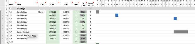
I have created a new GANNT chart, and am wanting the top row on each section to populate with the info of the section below, how does one do this please?
Thanks
I have created a new GANNT chart, and am wanting the top row on each section to populate with the info of the section below, how does one do this please?
Thanks
| gantt-chart_L.xlsx | ||||||||||||||||||||||||||||||||||||||||||||||||||||||
|---|---|---|---|---|---|---|---|---|---|---|---|---|---|---|---|---|---|---|---|---|---|---|---|---|---|---|---|---|---|---|---|---|---|---|---|---|---|---|---|---|---|---|---|---|---|---|---|---|---|---|---|---|---|---|
| A | B | C | E | F | G | H | I | J | K | L | M | N | O | P | Q | R | S | T | U | V | W | X | Y | Z | AA | AB | AC | AD | AE | AF | AG | AH | AI | AJ | AK | AL | AM | AN | AO | AP | AQ | AR | AS | AT | AU | AV | AW | AX | AY | AZ | ||||
| 4 | Project Start Date | 01/05/23 | Display Week | 1 | Week 1 | Week 2 | Week 3 | Week 4 | Week 5 | Week 6 | ||||||||||||||||||||||||||||||||||||||||||||
| 5 | Project Lead | 1 May 2023 | 8 May 2023 | 15 May 2023 | 22 May 2023 | 29 May 2023 | 5 Jun 2023 | |||||||||||||||||||||||||||||||||||||||||||||||
| 6 | 1 | 2 | 3 | 4 | 5 | 6 | 7 | 8 | 9 | 10 | 11 | 12 | 13 | 14 | 15 | 16 | 17 | 18 | 19 | 20 | 21 | 22 | 23 | 24 | 25 | 26 | 27 | 28 | 29 | 30 | 31 | 1 | 2 | 3 | 4 | 5 | 6 | 7 | 8 | 9 | 10 | 11 | ||||||||||||
| 7 | WBS | TASK | LEAD | START | END | DAYS | % DONE | WORK DAYS | M | T | W | T | F | S | S | M | T | W | T | F | S | S | M | T | W | T | F | S | S | M | T | W | T | F | S | S | M | T | W | T | F | S | S | M | T | W | T | F | S | S | ||||
| 8 | 1 | Holidays | - | - | ||||||||||||||||||||||||||||||||||||||||||||||||||
| 9 | 1.1 | Bank Holiday | [Name] | 01/05/23 | 01/05/23 | 1 | 100% | 1 | ||||||||||||||||||||||||||||||||||||||||||||||
| 10 | 1.2 | Bank Holiday | 08/05/23 | 08/05/23 | 1 | 60% | 1 | |||||||||||||||||||||||||||||||||||||||||||||||
| 11 | 1.3 | Bank Holiday | 29/05/23 | 29/05/23 | 1 | 0% | 1 | |||||||||||||||||||||||||||||||||||||||||||||||
| 12 | 1.4 | Bank Holiday | 28/08/23 | 28/08/23 | 1 | 75% | 1 | |||||||||||||||||||||||||||||||||||||||||||||||
| 13 | 1.5 | Bank Holiday | 25/12/23 | 25/12/23 | 1 | 0% | 1 | |||||||||||||||||||||||||||||||||||||||||||||||
| 14 | 1.6 | Bank Holiday | 26/12/23 | 26/12/23 | 1 | 0% | 1 | |||||||||||||||||||||||||||||||||||||||||||||||
| 15 | 1.7 | School Holidays | 29/05/23 | 02/06/23 | 5 | 100% | 5 | |||||||||||||||||||||||||||||||||||||||||||||||
| 16 | 1.8 | Scottish Bank Holiday | 07/08/23 | 07/08/23 | 1 | 200% | 1 | |||||||||||||||||||||||||||||||||||||||||||||||
| 17 | 1.9 | Bank Holiday | 30/11/23 | 30/11/23 | 1 | 300% | 1 | |||||||||||||||||||||||||||||||||||||||||||||||
| 18 | 1.10 | 0 | 400% | |||||||||||||||||||||||||||||||||||||||||||||||||||
| 19 | 1.11 | - | 0% | - | ||||||||||||||||||||||||||||||||||||||||||||||||||
GanttChart | ||||||||||||||||||||||||||||||||||||||||||||||||||||||
| Cell Formulas | ||
|---|---|---|
| Range | Formula | |
| K4,R4,Y4,AF4,AM4,AT4 | K4 | ="Week "&(K6-($C$4-WEEKDAY($C$4,1)+2))/7+1 |
| K5,R5,Y5,AF5,AM5,AT5 | K5 | =K6 |
| K6 | K6 | =C4-WEEKDAY(C4,1)+2+7*(H4-1) |
| L6:AZ6 | L6 | =K6+1 |
| K7:AZ7 | K7 | =CHOOSE(WEEKDAY(K6,1),"S","M","T","W","T","F","S") |
| F8 | F8 | =IF(ISBLANK(E8)," - ",IF(G8=0,E8,E8+G8-1)) |
| I8:I17,I19 | I8 | =IF(OR(F8=0,E8=0)," - ",NETWORKDAYS(E8,F8)) |
| A8 | A8 | =IF(ISERROR(VALUE(SUBSTITUTE(prevWBS,".",""))),"1",IF(ISERROR(FIND("`",SUBSTITUTE(prevWBS,".","`",1))),TEXT(VALUE(prevWBS)+1,"#"),TEXT(VALUE(LEFT(prevWBS,FIND("`",SUBSTITUTE(prevWBS,".","`",1))-1))+1,"#"))) |
| A9:A19 | A9 | =IF(ISERROR(VALUE(SUBSTITUTE(prevWBS,".",""))),"0.1",IF(ISERROR(FIND("`",SUBSTITUTE(prevWBS,".","`",1))),prevWBS&".1",LEFT(prevWBS,FIND("`",SUBSTITUTE(prevWBS,".","`",1)))&IF(ISERROR(FIND("`",SUBSTITUTE(prevWBS,".","`",2))),VALUE(RIGHT(prevWBS,LEN(prevWBS)-FIND("`",SUBSTITUTE(prevWBS,".","`",1))))+1,VALUE(MID(prevWBS,FIND("`",SUBSTITUTE(prevWBS,".","`",1))+1,(FIND("`",SUBSTITUTE(prevWBS,".","`",2))-FIND("`",SUBSTITUTE(prevWBS,".","`",1))-1)))+1))) |
| G9:G19 | G9 | =I9 |
| Cells with Conditional Formatting | ||||
|---|---|---|---|---|
| Cell | Condition | Cell Format | Stop If True | |
| H8:H45 | Other Type | DataBar | NO | |
| BO6:RR7,K6:BN45 | Expression | =K$6=TODAY() | text | NO |
| K6:RR7 | Expression | =K$6=TODAY() | text | NO |
| K8:BN45 | Expression | =AND($E8<=K$6,ROUNDDOWN(($F8-$E8+1)*$H8,0)+$E8-1>=K$6) | text | NO |
| K8:BN45 | Expression | =AND(NOT(ISBLANK($E8)),$E8<=K$6,$F8>=K$6) | text | NO |
| Cells with Data Validation | ||
|---|---|---|
| Cell | Allow | Criteria |
| H4 | Any value | |