with this macro
VBA Code:
Sub Insert_row()
Dim iRow As Long, LstRw1 As Long, LstRw2 As Long
Dim LstCol As Integer
Application.ScreenUpdating = False
LstRw1 = Range("A" & Rows.Count).End(xlUp).Row
For iRow = LstRw1 To 3 Step -1 '<~~ this is the magic
Cells(iRow, 1).EntireRow.Insert Shift:=xlDown
Next iRow
LstRw2 = Range("A" & Rows.Count).End(xlUp).Row + 1
LstCol = Cells(2, Columns.Count).End(xlToLeft).Column
With Range(Cells(2, 3), Cells(LstRw2, LstCol))
.SpecialCells(4).FormulaR1C1 = _
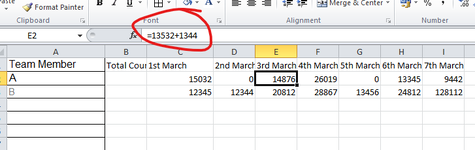
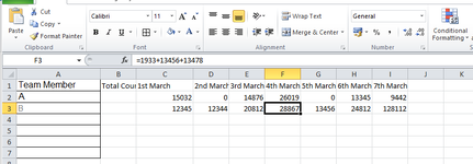
"=IFNA(IF(R[-1]C<>0,LEN(FORMULATEXT(R[-1]C))-LEN(SUBSTITUTE(FORMULATEXT(R[-1]C),""+"","""")),0),0)+IF(R[-1]C<>0,1,0)"
End With
Range(Cells(2, 1), Cells(LstRw2, 1)).SpecialCells(xlCellTypeConstants, 23).Offset(, 1).FormulaR1C1 = "=SUM(R[1]C[1]:R[1]C" & LstCol & ")"
Application.ScreenUpdating = True
End Sub
but I have no idea what the code would be for Google Sheets
Thank you for quick help mark. Taking inspiration from your last shared formula, i rather repeated the formula for 31 columns (depicting days) and it worked. =IFNA(IF(K2<>0,LEN(FORMULATEXT(K2))-LEN(SUBSTITUTE(FORMULATEXT(K2),"+","")),0),0)+IF(K2<>0,1,0) +IFNA(IF(L2<>0,LEN(FORMULATEXT(L2))-LEN(SUBSTITUTE(FORMULATEXT(L2),"+","")),0),0)+IF(L2<>0,1,0) +IFNA(IF(M2<>0,LEN(FORMULATEXT(M2))-LEN(SUBSTITUTE(FORMULATEXT(M2),"+","")),0),0)+IF(M2<>0,1,0) +IFNA(IF(N2<>0,LEN(FORMULATEXT(N2))-LEN(SUBSTITUTE(FORMULATEXT(N2),"+","")),0),0)+IF(N2<>0,1,0) +IFNA(IF(O2<>0,LEN(FORMULATEXT(O2))-LEN(SUBSTITUTE(FORMULATEXT(O2),"+","")),0),0)+IF(O2<>0,1,0) +IFNA(IF(P2<>0,LEN(FORMULATEXT(P2))-LEN(SUBSTITUTE(FORMULATEXT(P2),"+","")),0),0)+IF(P2<>0,1,0) +IFNA(IF(Q2<>0,LEN(FORMULATEXT(Q2))-LEN(SUBSTITUTE(FORMULATEXT(Q2),"+","")),0),0)+IF(Q2<>0,1,0) +IFNA(IF(R2<>0,LEN(FORMULATEXT(R2))-LEN(SUBSTITUTE(FORMULATEXT(R2),"+","")),0),0)+IF(R2<>0,1,0) +IFNA(IF(S2<>0,LEN(FORMULATEXT(S2))-LEN(SUBSTITUTE(FORMULATEXT(S2),"+","")),0),0)+IF(S2<>0,1,0) +IFNA(IF(T2<>0,LEN(FORMULATEXT(T2))-LEN(SUBSTITUTE(FORMULATEXT(T2),"+","")),0),0)+IF(T2<>0,1,0) +IFNA(IF(U2<>0,LEN(FORMULATEXT(U2))-LEN(SUBSTITUTE(FORMULATEXT(U2),"+","")),0),0)+IF(U2<>0,1,0) +IFNA(IF(V2<>0,LEN(FORMULATEXT(V2))-LEN(SUBSTITUTE(FORMULATEXT(V2),"+","")),0),0)+IF(V2<>0,1,0) +IFNA(IF(W2<>0,LEN(FORMULATEXT(W2))-LEN(SUBSTITUTE(FORMULATEXT(W2),"+","")),0),0)+IF(W2<>0,1,0) +IFNA(IF(X2<>0,LEN(FORMULATEXT(X2))-LEN(SUBSTITUTE(FORMULATEXT(X2),"+","")),0),0)+IF(X2<>0,1,0) +IFNA(IF(Y2<>0,LEN(FORMULATEXT(Y2))-LEN(SUBSTITUTE(FORMULATEXT(Y2),"+","")),0),0)+IF(Y2<>0,1,0) +IFNA(IF(Z2<>0,LEN(FORMULATEXT(Z2))-LEN(SUBSTITUTE(FORMULATEXT(Z2),"+","")),0),0)+IF(Z2<>0,1,0) +IFNA(IF(AA2<>0,LEN(FORMULATEXT(AA2))-LEN(SUBSTITUTE(FORMULATEXT(AA2),"+","")),0),0)+IF(AA2<>0,1,0) +IFNA(IF(AB2<>0,LEN(FORMULATEXT(AB2))-LEN(SUBSTITUTE(FORMULATEXT(AB2),"+","")),0),0)+IF(AB2<>0,1,0) +IFNA(IF(AC2<>0,LEN(FORMULATEXT(AC2))-LEN(SUBSTITUTE(FORMULATEXT(AC2),"+","")),0),0)+IF(AC2<>0,1,0) +IFNA(IF(AD2<>0,LEN(FORMULATEXT(AD2))-LEN(SUBSTITUTE(FORMULATEXT(AD2),"+","")),0),0)+IF(AD2<>0,1,0) +IFNA(IF(AE2<>0,LEN(FORMULATEXT(AE2))-LEN(SUBSTITUTE(FORMULATEXT(AE2),"+","")),0),0)+IF(AE2<>0,1,0) +IFNA(IF(AF2<>0,LEN(FORMULATEXT(AF2))-LEN(SUBSTITUTE(FORMULATEXT(AF2),"+","")),0),0)+IF(AF2<>0,1,0) +IFNA(IF(AG2<>0,LEN(FORMULATEXT(AG2))-LEN(SUBSTITUTE(FORMULATEXT(AG2),"+","")),0),0)+IF(AG2<>0,1,0) +IFNA(IF(AH2<>0,LEN(FORMULATEXT(AH2))-LEN(SUBSTITUTE(FORMULATEXT(AH2),"+","")),0),0)+IF(AH2<>0,1,0) +IFNA(IF(AM2<>0,LEN(FORMULATEXT(AM2))-LEN(SUBSTITUTE(FORMULATEXT(AM2),"+","")),0),0)+IF(AM2<>0,1,0) +IFNA(IF(AN2<>0,LEN(FORMULATEXT(AN2))-LEN(SUBSTITUTE(FORMULATEXT(AN2),"+","")),0),0)+IF(AN2<>0,1,0) +IFNA(IF(AO2<>0,LEN(FORMULATEXT(AO2))-LEN(SUBSTITUTE(FORMULATEXT(AO2),"+","")),0),0)+IF(AO2<>0,1,0) +IFNA(IF(AP2<>0,LEN(FORMULATEXT(AP2))-LEN(SUBSTITUTE(FORMULATEXT(AP2),"+","")),0),0)+IF(AP2<>0,1,0) +IFNA(IF(AQ2<>0,LEN(FORMULATEXT(AQ2))-LEN(SUBSTITUTE(FORMULATEXT(AQ2),"+","")),0),0)+IF(AQ2<>0,1,0) +IFNA(IF(AR2<>0,LEN(FORMULATEXT(AR2))-LEN(SUBSTITUTE(FORMULATEXT(AR2),"+","")),0),0)+IF(AR2<>0,1,0)
Thank you so much again.