How to apply mass conditional formatting with a formula

Revvy

New Member
Joined
Jul 11, 2022
Messages
5
Office Version
  1. 365
Platform
  1. Windows
Hi all

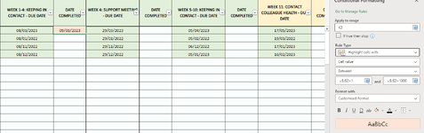
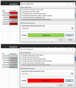
Im trying to make a conditional format that will turn a cell either green or red, depending on if it is equal to or greater than the cell next to it.

In this case its a date, if a task has been completed in time i want it green, and if it was completed late to turn red.

Ive achieved this in one cell, but cannot make it apply to the entire row to always use the cell next to it.

All help appreciated, im very self taught and have big gaps in my excel knowledge!
 

Attachments

  • Capture.PNG
    Capture.PNG
    52 KB · Views: 10

Excel Facts

Copy PDF to Excel
Select data in PDF. Paste to Microsoft Word. Copy from Word and paste to Excel.
Hi,
Which are the Columns you need to format ?
What is the rule you want to apply ?
 
Upvote 0
I created this macro after having recorded myself applying the 2 different conditional formats. Since I don't know the specific column(s) you want to utilize, I dummied up some data in Columns G and H and crafted this macro based on adding conditional formatting to cells H4:H9; you'll need to alter the formulas to reflect the proper column(s).

VBA Code:
Sub ConditionTheFOuttaThemCells()

With Selection

  .FormatConditions.Add _
    Type:=xlExpression, _
    Formula1:="=$H4>$G4"
  
  .FormatConditions(Selection.FormatConditions.Count).SetFirstPriority
  
  With .FormatConditions(1).Interior
  
   .Color = vbRed
  
  End With
  
  .FormatConditions(1).StopIfTrue = False

  .FormatConditions.Add _
    Type:=xlExpression, _
    Formula1:="=$H4<$G4"
  
  .FormatConditions(Selection.FormatConditions.Count).SetFirstPriority
  
  With .FormatConditions(1).Interior
  
   .Color = vbGreen
  
  End With
  
  .FormatConditions(1).StopIfTrue = False


End With


End Sub
 

Attachments

  • MrExcel0309_2.png
    MrExcel0309_2.png
    147.7 KB · Views: 7
Upvote 0
Im trying to make a conditional format
We cannot actually see your column or row labels so you may have to adjust, but for my layout below, I selected all the way from C2 (that is, the top-left 'Date Completed' cell) across and down to G10 (what I decided might be my bottom-right 'Date Completed' cell) and applied the Conditional Formatting shown.

23 03 11.xlsm
BCDEFG
1Week ..DATE COMPLETEDWeek ..DATE COMPLETEDWeek ..DATE COMPLETED
28/03/20239/03/202329/03/20235/04/2023
38/01/202229/01/202225/12/20215/02/2022
48/11/202229/11/202229/11/20226/12/2022
58/12/202229/11/20225/01/20237/03/2023
6
7
8
9
10
Red Green
Cells with Conditional Formatting
CellConditionCell FormatStop If True
C2:G10Expression=AND(LEFT(C$1,4)="DATE",C2<>"",C2<=B2)textNO
C2:G10Expression=AND(LEFT(C$1,4)="DATE",C2<>"",C2>B2)textNO
 
Upvote 0

Forum statistics

Threads
1,214,991
Messages
6,122,628
Members
449,095
Latest member
bsb1122

We've detected that you are using an adblocker.

We have a great community of people providing Excel help here, but the hosting costs are enormous. You can help keep this site running by allowing ads on MrExcel.com.
Allow Ads at MrExcel

Which adblocker are you using?

Disable AdBlock

Follow these easy steps to disable AdBlock

1)Click on the icon in the browser’s toolbar.
2)Click on the icon in the browser’s toolbar.
2)Click on the "Pause on this site" option.
Go back

Disable AdBlock Plus

Follow these easy steps to disable AdBlock Plus

1)Click on the icon in the browser’s toolbar.
2)Click on the toggle to disable it for "mrexcel.com".
Go back

Disable uBlock Origin

Follow these easy steps to disable uBlock Origin

1)Click on the icon in the browser’s toolbar.
2)Click on the "Power" button.
3)Click on the "Refresh" button.
Go back

Disable uBlock

Follow these easy steps to disable uBlock

1)Click on the icon in the browser’s toolbar.
2)Click on the "Power" button.
3)Click on the "Refresh" button.
Go back
Back
Top