How to copy rows from one worksheet to a new worksheet if a cell matches a cell from anothe worksheet

DennisYoung

New Member
Joined
Jun 27, 2022
Messages
14
Office Version
  1. 2021
  2. 2016
Platform
  1. Windows
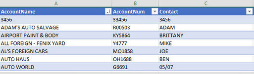
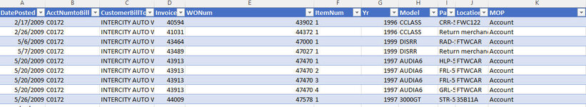
What I am trying to accomplish is, I have 3 worksheets, sheet 1 and sheet 2, and sheet3, Column B of worksheet 1 is account number, column B of worksheet 2 is also account number, worksheet 3 is currently blank. I want to compare column B of WS 2 with column B of WS1 and if WS2 matches the account number in WS1 then copy that entire row from WS2 to WS3 first available row and so forth.
 

Attachments

  • Screenshot1.jpg
    Screenshot1.jpg
    37.5 KB · Views: 9
  • Screenshot2.jpg
    Screenshot2.jpg
    101.3 KB · Views: 8

Excel Facts

Do you hate GETPIVOTDATA?
Prevent GETPIVOTDATA. Select inside a PivotTable. In the Analyze tab of the ribbon, open the dropown next to Options and turn it off
Try the following on a copy of your workbook - just change the sheet names in the code to suit.

VBA Code:
Option Explicit
Sub DennisYoung()
    Dim ws1 As Worksheet, ws2 As Worksheet, ws3 As Worksheet
    Set ws1 = Worksheets("Sheet1")  '<~~ *** Change sheet names to actual sheet names ***
    Set ws2 = Worksheets("Sheet2")
    Set ws3 = Worksheets("Sheet3")
    
    Dim a, i As Long
    a = ws1.Range("B2:B" & ws1.Cells(Rows.Count, "B").End(xlUp).Row).Value
    a = Application.Transpose(Application.Index(a, 0, 1))
    For i = LBound(a) To UBound(a)
        a(i) = CStr(a(i))
    Next i
    
    With ws2.Range("A1").CurrentRegion
        .AutoFilter 2, Array(a), 7
        If ws2.Cells(Rows.Count, 1).End(xlUp).Row > 1 Then
            .Offset(1).Resize(.Rows.Count - 1).Copy ws3.Range("A" & ws3.Cells(Rows.Count, 1).End(xlUp).Row + 1)
        End If
        ws2.ShowAllData
    End With
End Sub
 
Upvote 0
Solution
Try the following on a copy of your workbook - just change the sheet names in the code to suit.

VBA Code:
Option Explicit
Sub DennisYoung()
    Dim ws1 As Worksheet, ws2 As Worksheet, ws3 As Worksheet
    Set ws1 = Worksheets("Sheet1")  '<~~ *** Change sheet names to actual sheet names ***
    Set ws2 = Worksheets("Sheet2")
    Set ws3 = Worksheets("Sheet3")
   
    Dim a, i As Long
    a = ws1.Range("B2:B" & ws1.Cells(Rows.Count, "B").End(xlUp).Row).Value
    a = Application.Transpose(Application.Index(a, 0, 1))
    For i = LBound(a) To UBound(a)
        a(i) = CStr(a(i))
    Next i
   
    With ws2.Range("A1").CurrentRegion
        .AutoFilter 2, Array(a), 7
        If ws2.Cells(Rows.Count, 1).End(xlUp).Row > 1 Then
            .Offset(1).Resize(.Rows.Count - 1).Copy ws3.Range("A" & ws3.Cells(Rows.Count, 1).End(xlUp).Row + 1)
        End If
        ws2.ShowAllData
    End With
End Sub
Thank you very much! Worked like a charm.
 
Upvote 0

Forum statistics

Threads
1,215,575
Messages
6,125,631
Members
449,241
Latest member
NoniJ

We've detected that you are using an adblocker.

We have a great community of people providing Excel help here, but the hosting costs are enormous. You can help keep this site running by allowing ads on MrExcel.com.
Allow Ads at MrExcel

Which adblocker are you using?

Disable AdBlock

Follow these easy steps to disable AdBlock

1)Click on the icon in the browser’s toolbar.
2)Click on the icon in the browser’s toolbar.
2)Click on the "Pause on this site" option.
Go back

Disable AdBlock Plus

Follow these easy steps to disable AdBlock Plus

1)Click on the icon in the browser’s toolbar.
2)Click on the toggle to disable it for "mrexcel.com".
Go back

Disable uBlock Origin

Follow these easy steps to disable uBlock Origin

1)Click on the icon in the browser’s toolbar.
2)Click on the "Power" button.
3)Click on the "Refresh" button.
Go back

Disable uBlock

Follow these easy steps to disable uBlock

1)Click on the icon in the browser’s toolbar.
2)Click on the "Power" button.
3)Click on the "Refresh" button.
Go back
Back
Top