How to merge multiple tables using SUMPRODUCT and Start:End ?

[sprunknwn]

Hi there,

I have a sheet for each week that contains the same table and a sheet for Totals.
I created two blank sheets (Start and End) and I use them to sum up the stats I have from all sheets in between in the totals sheet table.
For example -
=SUM(Start:End!C2) - This sums up all C2 cells from all tables in sheets between Start and End into C2 in the totals sheet table.
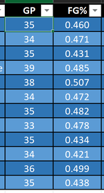
Every table has a GP(games played) column and FG%(field goal %).

What I would like to do is to multiply the FG% and the GP column for each table row and then sum it up, eventually dividing it by the total amount of games played.
When I used the aforementioned SUM function, it works just fine.
When I try to do the same with the following -
=SUMPRODUCT(Start:End!C2,Start:End!D2)
I keep getting either NAME error, REF error.
I tried all sorts of syntax but can't quite get the right one -
=SUMPRODUCT(Start:End!C2:C13,Start:End!D2:D13)
=SUMPRODUCT(Start:End!C:C,Start:End!D:D)
=SUM(SUMPRODUCT(Start:End!C2:C13,Start:End!D2:D13))

Just can't seem to find the correct syntax.
Any assistance will be appreciated and if something is not clear, feel free to ask.

Thanks in advance!

 

[jasonb75]

Welcome to Mr Excel!

Unfortunately, there appears no way (with current functions) of performing a 3d sumproduct calculation in the ways that you are trying.

The closest thing that you could get would be something on the basis of

=SUM(SUMIF(INDIRECT("'"&Sheetlist&"'!RC3",0),"<>0")*SUMIF(INDIRECT("'"&Sheetlist&"'!RC4",0),"<>0"))

which is the equivalent to the first formula that you tried,

=SUMPRODUCT(Start:End!C2,Start:End!D2)

It is not possible to use multiple sheets and ranges of more than 1 cell in this way (except with basic counts / sums).

Note that you will not be able to use Start:End for this formula, it needs a full list of the individual sheet names to work with. In the example formula, I have used a named range called 'Sheetlist' which contains all of the relevant sheet names for the formula to use.

Also, because of the way that the INDIRECT function works it is necessary to use R1C1 notation so that the row increases when you drag the formula down. I've assumed that the formula will be starting in row 2. If it is not then that will need some adjustment.

It's not what I would consider an ideal solution but is the only thing that will work for what you need.

 

[sprunknwn]

Hey Jason,

Thank you so much for taking the time to answer my question.
A few more questions if you will (please excuse me if they seem too basic).
How do I create a parameter that contains all sheet names to replace "sheetlist"? (or did I misunderstand the syntax there?)
Also, If the rows with values start in the second row, the GP column is C and FG% is D, the command would be -

=SUM(SUMIF(INDIRECT("'"&Sheetlist&"'![B]RC2"[/B],0),"<>0")*SUMIF(INDIRECT("'"&Sheetlist&"'![B]RD2[/B]",0),"<>0"))

Thanks again!

 

[sprunknwn]

Hey Jason,

Thank you so much for taking the time to answer my question.
A few more questions if you will (please excuse me if they seem too basic).
How do I create a parameter that contains all sheet names to replace "sheetlist"? (or did I misunderstand the syntax there?)
Also, If the rows with values start in the second row, the GP column is C and FG% is D, the command would be -

=SUM(SUMIF(INDIRECT("'"&Sheetlist&"'![B]RC2"[/B],0),"<>0")*SUMIF(INDIRECT("'"&Sheetlist&"'![B]RD2[/B]",0),"<>0"))

Thanks again!

Disregard the .
I just wanted to make the RC2 and RD2 bold.

 

[sprunknwn]

Disregard the [ B ] [ / B ] part in the formula.

 

[jasonb75]

How do I create a parameter that contains all sheet names to replace "sheetlist"? (or did I misunderstand the syntax there?)

For this part, the easy way is to make a list in a dedicated sheet, with your sheet names in say A2:A10 then create a named range that refers to A1:A10 in that sheet.
To the left of the formula bar you will see a smaller box that contains the address of the selected cell. Selecting the range that you want to name, then typing the name (Sheetname) into that box creates the name for you.

Also, If the rows with values start in the second row, the GP column is C and FG% is D, the command would be -

For that, it would be as I had written it. "RC3" and "RC4" respectively. R (without a number) indicates the same row as the formula. C3 indicates column 3, C4 indicates column 4, and so on.
The numbers entered like that mean a fixed column (or row) the same as using $ signs in a normal formula. If you enter the numbers in square brackets then it is relative to the cell with the formula. R[-1] means row above R[1] is the row below C[-1] column to the left and C[1] column to the right. There are probably far better explanations than mine out there if you search Excel R1C1 notation.

Disregard the [ B ] [ / B ] part in the formula.

If you want to apply formatting to formulas / code to highlight a specific part then I think that you need to use the </>Rich icon (it's been a while since I've needed to so I might have the wrong one).

Hopefully that makes sense, if you need me to clarify anything I'll be here on and off for a few more hours.

 

[sprunknwn]

Hey Jason, sorry for the lack of response.
I somehow lost all my data and had to recover it (manually fill in the tables).
I think I understand the formula better but it seems like that's not exactly what I had in mind, I'll explain.
Each Sheet is a Week of stats where I have GP (games played) column and a total FG% for the week.
So lets say team "Spr" had 10GP on 50% in week one, and 10GP on 30% week two.
The calculation should be as followed -
(GPWK1 * FG%WK1) + (GPWK2 * FG%WK2) / Total GP
(10*0.50 + 10*0.3) / 20 = 0.4
So the total FG% for team "Spr" is 40% or 0.400.
How can I do this calculation with the option to add another sheet for each upcoming week?

Thanks a bunch!

 

[sprunknwn]

I followed the evaluation of the formula, and it seems for the most part that it does do what I need but, there is a REF error at the end that I just can't figure out.
A REF error coming from the table in Week4.
I will try to see what's going on but essentially, it works.

Thanks a lot Jason!

 

[jasonb75]

A ref error means that the range doesn't exist. If you have followed the steps that i suggested and listed the sheets to a named range then it must only include sheets that exist, no names for sheets that you might be adding later and no empty cells. If the range contains either of those things then it will cause the error.

 

[sprunknwn]

You're right.
Sheet 4 had a space in the name(Week 4) while the Sheetlist did not(Week4).

Thanks again, works perfectly!