If cell is 0, try next cell. If that cell is 0, try 2 cells over; do so until value is found

gilbertjay07

New Member
Joined
Aug 22, 2023
Messages
3
Office Version
  1. 365
Platform
  1. Windows
Hello,

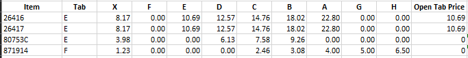
I could really use some help with this formula. What I'm trying to do is take the value in column B (called "Tab") and match it to the corresponding value in the table (columns G:O).

For example, the first item's value would be 10.69.
I'm currently using INDEX to match this value to the correct item, here is my formula: =INDEX(G8:O8,1,IF(B8="X",1,IF(B8="F",2,IF(B8="E",3,IF(B8="D",4,IF(B8="C",5,IF(B8="B",6,IF(B8="A",7,IF(B8="G",8,9)))))))))​

But when the value returned is 0, it should return the next column's value, as seen with item 80753C.
=IF(P10=0,INDEX(G10:O10,1,(IF(B10="X",1,IF(B10="F",2,IF(B10="E",3,IF(B10="D",4,IF(B10="C",5,IF(B10="B",6,IF(B10="A",7,IF(B10="G",8,9)))))))))+1),P10)​

The problem I have is for item 871914. It is at F tab, which is 0 (F11), so the current formula that I'm using would return the value from E11, which is 0 in this case. How can I have it repeatedly check the next cell over until it returns a value greater than 0 (C11 in this case)?

Return value.PNG
 

Attachments

  • Return value.PNG
    Return value.PNG
    6.2 KB · Views: 5

Excel Facts

Move date out one month or year
Use =EDATE(A2,1) for one month later. Use EDATE(A2,12) for one year later.
Hi & welcome to MrExcel.
How about
Excel Formula:
=LET(a,DROP(G8:O8,,XMATCH(B8,$G$7:$O$7)),TAKE(FILTER(a,a<>0),,1))
 
Upvote 0
Hi & welcome to MrExcel.
How about
Excel Formula:
=LET(a,DROP(G8:O8,,XMATCH(B8,$G$7:$O$7)),TAKE(FILTER(a,a<>0),,1))
See what I miss when I don't play with new toys in the last couple years. That is so much nicer than this monster:

Excel Formula:
=INDEX(OFFSET($G8,0,MATCH($B8,$G$7:$O$7,0)-1,,10-MATCH($B8,$G$7:$O$7,0)),1,MATCH(TRUE,OFFSET($G8,0,MATCH($B8,$G$7:$O$7,0)-1,,10-MATCH($B8,$G$7:$O$7,0))<>0,0))

However, I might mention your formula is returning different results than mine for rows 8 and 9. When I use yours, I get 12.57 instead of 10.69. Thoughts?
 
Upvote 0
Forgot to subtract 1, it should be
Excel Formula:
=LET(a,DROP(G8:O8,,XMATCH(B8,$G$7:$O$7)-1),TAKE(FILTER(a,a<>0),,1))
 
Upvote 1
Solution
Forgot to subtract 1, it should be
Excel Formula:
=LET(a,DROP(G8:O8,,XMATCH(B8,$G$7:$O$7)-1),TAKE(FILTER(a,a<>0),,1))
This worked (with the subtract 1) - I can't begin to thank you enough, I really appreciate your help!
 
Upvote 0
Glad we could help & thanks for the feedback.
Would you be able to show me the formula that would display the new tab that was selected (if it differs from the original tab) - for example, item 871914 is no longer tab F, but is now tab C. Ideally, I would like to have a new column that shows the new tab is C.
 
Upvote 0
If you change B11 to C then the formula will show the the value from that column.
 
Upvote 0

Forum statistics

Threads
1,215,085
Messages
6,123,030
Members
449,092
Latest member
ikke

We've detected that you are using an adblocker.

We have a great community of people providing Excel help here, but the hosting costs are enormous. You can help keep this site running by allowing ads on MrExcel.com.
Allow Ads at MrExcel

Which adblocker are you using?

Disable AdBlock

Follow these easy steps to disable AdBlock

1)Click on the icon in the browser’s toolbar.
2)Click on the icon in the browser’s toolbar.
2)Click on the "Pause on this site" option.
Go back

Disable AdBlock Plus

Follow these easy steps to disable AdBlock Plus

1)Click on the icon in the browser’s toolbar.
2)Click on the toggle to disable it for "mrexcel.com".
Go back

Disable uBlock Origin

Follow these easy steps to disable uBlock Origin

1)Click on the icon in the browser’s toolbar.
2)Click on the "Power" button.
3)Click on the "Refresh" button.
Go back

Disable uBlock

Follow these easy steps to disable uBlock

1)Click on the icon in the browser’s toolbar.
2)Click on the "Power" button.
3)Click on the "Refresh" button.
Go back
Back
Top