IF FORMULA GONE WRONG

EXCELTRBLD

New Member
Joined
Feb 22, 2024
Messages
4
Office Version
  1. 365
Platform
  1. Windows
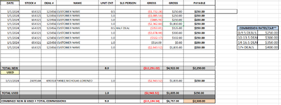
Hello, can someone assist with the below formula? I'm using this formula, but it's not recognizing the "unit cnt" if it's 0.5 it doesn't give me half of the "payable" amount or it it's a "0" it doesn't change the "payable to $0.00. What can I add or remove from the formula below so it recognizes the "unit cnt"?

=CEILING(IF(G8=0,0,IF($G$34<10,$L$37,IF($G$34<14,$L$38,IF($G$34<17,$L$39,IF($G$34>16.5,L$40))))),0.01)
 

Attachments

  • COMMISSION_Template.png
    COMMISSION_Template.png
    60.6 KB · Views: 9

Excel Facts

Highlight Duplicates
Home, Conditional Formatting, Highlight Cells, Duplicate records, OK to add pink formatting to any duplicates in selected range.
Your screenshot doesn't tell us where the data is located (row and column references) or which cell is supposed to contain the formula. Could you share the data using XL2BB or as a table with column and row identifiers? It would also help if you provide some cells with expected results shown.
 
Upvote 0
I was able to paste the table below. Hope you can assist. Thank you!!!
DATESTOCK #DEAL #NAMEUNIT CNTSPLIT/PERSONGROSSGROSSPAYABLE
1/1/2024​
654321
123456​
CUSTOMER NAME
0.5​
($1,732.28)​
$250.00​
$250.00
1/1/2024​
654321
123456​
CUSTOMER NAME
1.0​
($1,085.54)​
$250.00​
$250.00
1/1/2024​
654321
123456​
CUSTOMER NAME
1.0​
($885.96)​
$250.00​
$250.00
1/1/2024​
654321
123456​
CUSTOMER NAME
1.0​
($2,362.84)​
$1,810.00​
$250.00
1/1/2024​
654321
123456​
CUSTOMER NAME
0.5​
HALF DEAL
($353.81)​
$125.00​
$250.00
1/1/2024​
654321
123456​
CUSTOMER NAME
1.0​
($3,078.99)​
$300.00​
$250.00
1/1/2024​
654321
123456​
CUSTOMER NAME
1.0​
($322.17)​
$102.00​
$250.00
1/1/2024​
654321
123456​
CUSTOMER NAME
1.0​
$514.09​
$0.00​
$250.00
1/1/2024​
654321
123456​
CUSTOMER NAME
1.0​
($322.17)​
$102.00​
$250.00
1/1/2024​
654321
123456​
CUSTOMER NAME
1.0​
$514.09​
$0.00​
$250.00
TOTAL NEW
9.0​
($9,115.58)$3,189.00$2,500.00
USED
 
Upvote 0
Where on the sheet are the cells? For instance, Is the cell labelled "DATE" in cell A1 or somewhere else? And where is the formula from your first post located?
 
Upvote 0
This is a bigger picture, the formula =IF($G$34<=10,$N$13,IF($G$34<=14,$N$14,IF($G$34<=17,$N$15,IF($G$34>=16.5,N$16)))) is in column "K"... I need it to show if column "G" shows a "0" or "0.5" unit count to make column "K" change the payable amount to either $0 or if it's 0.5 unit count to show half the payable amount. See image below it shows formula, and selected cells. I really appreciate any input. Thank you!!!
1708699954358.png
 
Upvote 0
You can just multiply the result of your full IF statement by the unit count cell.
Excel Formula:
=IF($G$39<=10,$N$13,IF($G$34<=14,$N$14,IF($G$34<=17,$N$15,IF($G$34>=16.5,$N$16))))*$G8
2024-02-22.xlsx
CDEFGHIJKLMN
6DATESTOCK #DEAL #NAMEUNIT CNTSPLIT/PERSONGROSSGROSSPAYABLE
7$0.00
801-01-24654321123456CUSTOMER NAME0.5$1,732.28$250.00$125.00
901-01-24654321123456CUSTOMER NAME1$1,085.54$250.00$250.00
1001-01-24654321123456CUSTOMER NAME1$885.96$250.00$250.00
1101-01-24654321123456CUSTOMER NAME1$2,362.84$1,810.00$250.00
1201-01-24654321123456CUSTOMER NAME0.5Half Deal$353.81$125.00$125.00COMMISSION RATES/CAR**
1301-01-24654321123456CUSTOMER NAME1$3,078.99$300.00$250.000-9.5 DEALS$250.00
1401-01-24654321123456CUSTOMER NAME1$322.17$102.00$250.0010-13.5 DEALS$300.00
1501-01-24654321123456CUSTOMER NAME1$514.09$0.00$250.0014-16.5 DEALS$350.00
1601-01-24654321123456CUSTOMER NAME1$322.17$102.00$250.0017+ DEALS$400.00
1701-01-24654321123456CUSTOMER NAME1$514.09$0.00$250.00
18$0.00
19$0.00
20$0.00
21TOTAL NEW9.0$8,471.24$3,189.00$2,250.00
22USED$0.00
23$0.00
2401-01-24654321123456CUSTOMER NAME1.0$2,943.52$1,835.00$250.00
25$0.00
31$0.00
32TOTAL USED1.0$2,943.52$1,835.00$250.00
33
34COMBINED NEW & USED = TOTAL COMMISSIONS10.0$11,414.76$5,024.00$2,500.00
35
Sheet1
Cell Formulas
RangeFormula
G21,J21:K21G21=SUM(G8:G20)
I21I21=SUM(I7:I20)
K31,K22:K25,K7:K20K7=IF($G$39<=10,$N$13,IF($G$34<=14,$N$14,IF($G$34<=17,$N$15,IF($G$34>=16.5,$N$16))))*$G7
G32,I32:K32G32=SUM(G22:G31)
G34,I34:K34G34=SUM(G21,G32)
 
Upvote 0
Solution
Also, consider changing your commission table, and then modify your commission formula to reference it as below. The way you currently have your formula, it isn't using the rates in the table.

2024-02-22.xlsx
CDEFGHIJKLMNOP
6DATESTOCK #DEAL #NAMEUNIT CNTSPLIT/PERSONGROSSGROSSPAYABLE
7$0.00
801-01-24654321123456CUSTOMER NAME0.5$1,732.28$250.00$150.00
901-01-24654321123456CUSTOMER NAME1$1,085.54$250.00$300.00
1001-01-24654321123456CUSTOMER NAME1$885.96$250.00$300.00
1101-01-24654321123456CUSTOMER NAME1$2,362.84$1,810.00$300.00
1201-01-24654321123456CUSTOMER NAME0.5Half Deal$353.81$125.00$150.00COMMISSION RATES/CAR**LowerUpper
1301-01-24654321123456CUSTOMER NAME1$3,078.99$300.00$300.000-9.5 DEALS$250.0009.5
1401-01-24654321123456CUSTOMER NAME1$322.17$102.00$300.0010-13.5 DEALS$300.001013.5
1501-01-24654321123456CUSTOMER NAME1$514.09$0.00$300.0014-16.5 DEALS$350.001416.5
1601-01-24654321123456CUSTOMER NAME1$322.17$102.00$300.0017+ DEALS$400.0017
1701-01-24654321123456CUSTOMER NAME1$514.09$0.00$300.00
18$0.00
19$0.00
20$0.00
21TOTAL NEW9.0$8,471.24$3,189.00$2,700.00
22USED$0.00
23$0.00
2401-01-24654321123456CUSTOMER NAME1.0$2,943.52$1,835.00$300.00
25$0.00
31$0.00
32TOTAL USED1.0$2,943.52$1,835.00$300.00
33
34COMBINED NEW & USED = TOTAL COMMISSIONS10.0$11,414.76$5,024.00$3,000.00
Sheet1
Cell Formulas
RangeFormula
G21,J21:K21G21=SUM(G8:G20)
I21I21=SUM(I7:I20)
K31,K22:K25,K7:K20K7=IF($G$34<=$P$13,$N$13,IF($G$34<=$P$14,$N$14,IF($G$34<=$P$15,$N$15,IF($G$34>=O16,$N$16))))*$G7
G32,I32:K32G32=SUM(G22:G31)
G34,I34:K34G34=SUM(G21,G32)
 
Upvote 0
This worked perfectly!! Thank you so much, appreciate your assistance!!!
 
Upvote 0

Forum statistics

Threads
1,215,069
Messages
6,122,953
Members
449,095
Latest member
nmaske

We've detected that you are using an adblocker.

We have a great community of people providing Excel help here, but the hosting costs are enormous. You can help keep this site running by allowing ads on MrExcel.com.
Allow Ads at MrExcel

Which adblocker are you using?

Disable AdBlock

Follow these easy steps to disable AdBlock

1)Click on the icon in the browser’s toolbar.
2)Click on the icon in the browser’s toolbar.
2)Click on the "Pause on this site" option.
Go back

Disable AdBlock Plus

Follow these easy steps to disable AdBlock Plus

1)Click on the icon in the browser’s toolbar.
2)Click on the toggle to disable it for "mrexcel.com".
Go back

Disable uBlock Origin

Follow these easy steps to disable uBlock Origin

1)Click on the icon in the browser’s toolbar.
2)Click on the "Power" button.
3)Click on the "Refresh" button.
Go back

Disable uBlock

Follow these easy steps to disable uBlock

1)Click on the icon in the browser’s toolbar.
2)Click on the "Power" button.
3)Click on the "Refresh" button.
Go back
Back
Top