If formula with values between x and y

Linsie · Feb 29, 2024

Hi,
I am working on a weight ranking for my projects. I have worked out all the totals etc but now getting stuck on my IF formula. Would be grateful for some assistance as been looking at it a while now and cant see where I am going wrong.

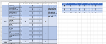
Some background. I have a chart where we have broken down the topics that will end up giving us a weight score. The sum total will tell us what the weight score is. ie if between 0-5 (0%) then the weight that should be returned is 0, between 5 and 10 (20%), then 1 should be returned and so on. Each weight is based on a %age of the points.

There is not any false statements on this, but if i took out the last ,"" then the formula would not work at all. Currently it just returns "FALSE" as the result.

The formula I was trying was (this is based on the Risk Category)
=IF(OR(G3=0,K3),IF(OR(G3>0,G3<5,K4),IF(OR(G3>5,G3<10,K5),IF(OR(G3>10,G3<15,K6),IF(OR(G3>15,G3<20,K7),IF(OR(G3>20,G3<25,K8),""))))))

Thanks in advance.

weighting.xlsx

A

B

C

D

E

F

G

H

I

J

K

L

M

N

O

P

Q

R

S

1

2

Keep

Total Points

SubCategory Points

Include or Not

Weight Points

Smartsheet Weight

Smartsheet Weigh

Score Value

Risk

Cost

Resouces

I&U

BV

T&D

Training

3

Risk

Compliance

Y

25

3

Y

15

FALSE

0

0%

0

4

DBA Team (Infosys)

Y

3

Y

1

20%

5

Export/Shipping

Y

3

Y

2

40%

6

Hardware Availability

Y

3

N

3

60%

7

Hot Works

Y

2

N

4

80%

8

Information Security

Y

3

N

5

100%

9

Microsoft Licensing

Y

2

N

10

Team Cooperation

Y

3

Y

11

WFMs

Y

3

Y

12

Costs

External Labour

Y

20

3

Y

14

13

Internal Labour

Y

2

Y

14

Licensing

Y

2

N

15

Maintenance

Y

3

Y

16

Power Consumption

Y

2

Y

17

Savings

Y

4

Y

18

Shipping

Y

4

N

19

Resources

Export

Y

20

2

Y

10

20

Hot works

Y

2

Y

21

ODCM

Y

2

N

22

OSES

Y

2

Y

23

OSS

Y

2

N

24

Other Teams ie DBA/IDN

Y

2

Y

25

Purchasing & Sourcing

Y

2

N

26

SD/MPG

Y

2

N

27

VDC

Y

2

Y

28

WFM

Y

2

N

29

Importance / Urgency

Budget

Y

15

4

Y

8

30

EOL

Y

4

Y

31

Strategic Need

Y

7

N

32

Business Value

Aligns with goals

Y

10

4

Y

7

33

Future Proofing

Y

3

N

34

Revenue

Y

3

Y

35

Time/Duration

Short - Up to 6 months

Y

5

2

Y

2

36

Long - 6+ Months

Y

3

N

37

Training

Not Required

Y

5

1

Y

1

38

Required

Y

4

N

Sheet2

Cell Formulas
Range	Formula
H3	H3	=IF(OR(G3=0,K3),IF(OR(G3>0,G3<5,K4),IF(OR(G3>5,G3<10,K5),IF(OR(G3>10,G3<15,K6),IF(OR(G3>15,G3<20,K7),IF(OR(G3>20,G3<25,K8),""))))))
M3:M8	M3	=$D$3*L3
N3:N8	N3	=$D$12*L3
O3:O8	O3	=$D$19*L3
P3:P8	P3	=$D$29*L3
Q3:Q8	Q3	=$D$32*L3
R3:R8	R3	=$D$35*L3
S3:S8	S3	=$D$37*L3
G3	G3	=SUMIF(F3:F11,"Y",E3:E11)
G12	G12	=SUMIF(F12:F18,"Y",E12:E18)
G19	G19	=SUMIF(F19:F28,"Y",E19:E28)
G29,G32	G29	=SUMIF(F29:F31,"Y",E29:E31)
G35,G37	G35	=SUMIF(F35:F36,"Y",E35:E36)

Asbestos_Jen · Feb 29, 2024

I think this does what you're after. Your original formula has the "result if true" condition inside of your "OR" statements, which is at least part of the problem. If you structure your IFs in ascending order, you shouldn't need the OR statements, as you'll always be comparing to a greater number at each step, and the IF will stop when it first encounters "true".

Book1

A

B

C

D

E

F

G

H

I

J

K

L

M

N

O

P

Q

R

S

1

2

Keep

Total Points

SubCategory Points

Include or Not

Weight Points

Smartsheet Weight

Smartsheet Weigh

Score Value

Risk

Cost

Resouces

I&U

BV

T&D

Training

3

Risk

Compliance

Y

25

3

Y

15

1

0

0%

0

4

DBA Team (Infosys)

Y

3

Y

1

20%

5

Export/Shipping

Y

3

Y

2

40%

6

Hardware Availability

Y

3

N

3

60%

7

Hot Works

Y

2

N

4

80%

8

Information Security

Y

3

N

5

100%

9

Microsoft Licensing

Y

2

N

10

Team Cooperation

Y

3

Y

11

WFMs

Y

3

Y

12

Costs

External Labour

Y

20

3

Y

14

1

13

Internal Labour

Y

2

Y

14

Licensing

Y

2

N

15

Maintenance

Y

3

Y

16

Power Consumption

Y

2

Y

17

Savings

Y

4

Y

18

Shipping

Y

4

N

19

Resources

Export

Y

20

2

Y

10

1

20

Hot works

Y

2

Y

21

ODCM

Y

2

N

22

OSES

Y

2

Y

23

OSS

Y

2

N

24

Other Teams ie DBA/IDN

Y

2

Y

25

Purchasing & Sourcing

Y

2

N

26

SD/MPG

Y

2

N

27

VDC

Y

2

Y

28

WFM

Y

2

N

Sheet1

Cell Formulas
Range	Formula
G3	G3	=SUMIF(F3:F11,"Y",E3:E11)
H3,H19,H12	H3	=IF(G3=0,0,IF(G3<=$L$4100,$K$4,IF(G3<=$L$5100,$K$5,IF(G3<=$L$6100,$K$6,IF(G3<=$L$7100,$K$7,IF(G3<=$L$8*100,$K$8,""))))))
G12	G12	=SUMIF(F12:F18,"Y",E12:E18)
G19	G19	=SUMIF(F19:F28,"Y",E19:E28)
M3:M8	M3	=$D$3*L3
N3:N8	N3	=$D$12*L3
O3:O8	O3	=$D$19*L3
P3:P8	P3	=$D$29*L3
Q3:Q8	Q3	=$D$32*L3
R3:R8	R3	=$D$35*L3
S3:S8	S3	=$D$37*L3
I8	I8	=IF(G3=0,0,IF(G3<=$L$4,$K$4,IF(G3<=$L$5,$K$5,IF(G3<=$L$6,$K$6,IF(G3<=$L$7,$K$7,IF(G3<=$L$8,$K$8,""))))))

Linsie · Feb 29, 2024

Asbestos_Jen said:
I think this does what you're after. Your original formula has the "result if true" condition inside of your "OR" statements, which is at least part of the problem. If you structure your IFs in ascending order, you shouldn't need the OR statements, as you'll always be comparing to a greater number at each step, and the IF will stop when it first encounters "true".

Book1
A B C D E F G H I J K L M N O P Q R S
1
2 Keep Total Points SubCategory Points Include or Not Weight Points Smartsheet Weight Smartsheet Weigh Score Value Risk Cost Resouces I&U BV T&D Training
3 Risk Compliance Y 25 3 Y 15 1 0 0% 0 0 0 0 0 0 0
4 DBA Team (Infosys) Y 3 Y 1 20% 5 4 4 3 2 1 1
5 Export/Shipping Y 3 Y 2 40% 10 8 8 6 4 2 2
6 Hardware Availability Y 3 N 3 60% 15 12 12 9 6 3 3
7 Hot Works Y 2 N 4 80% 20 16 16 12 8 4 4
8 Information Security Y 3 N 5 100% 25 20 20 15 10 5 5
9 Microsoft Licensing Y 2 N
10 Team Cooperation Y 3 Y
11 WFMs Y 3 Y
12 Costs External Labour Y 20 3 Y 14 1
13 Internal Labour Y 2 Y
14 Licensing Y 2 N
15 Maintenance Y 3 Y
16 Power Consumption Y 2 Y
17 Savings Y 4 Y
18 Shipping Y 4 N
19 Resources Export Y 20 2 Y 10 1
20 Hot works Y 2 Y
21 ODCM Y 2 N
22 OSES Y 2 Y
23 OSS Y 2 N
24 Other Teams ie DBA/IDN Y 2 Y
25 Purchasing & Sourcing Y 2 N
26 SD/MPG Y 2 N
27 VDC Y 2 Y
28 WFM Y 2 N
Sheet1
Cell Formulas
Range Formula
G3 G3 =SUMIF(F3:F11,"Y",E3:E11)
H3,H19,H12 H3 =IF(G3=0,0,IF(G3<=$L$4*100,$K$4,IF(G3<=$L$5*100,$K$5,IF(G3<=$L$6*100,$K$6,IF(G3<=$L$7*100,$K$7,IF(G3<=$L$8*100,$K$8,""))))))
G12 G12 =SUMIF(F12:F18,"Y",E12:E18)
G19 G19 =SUMIF(F19:F28,"Y",E19:E28)
M3:M8 M3 =$D$3*L3
N3:N8 N3 =$D$12*L3
O3:O8 O3 =$D$19*L3
P3:P8 P3 =$D$29*L3
Q3:Q8 Q3 =$D$32*L3
R3:R8 R3 =$D$35*L3
S3:S8 S3 =$D$37*L3
I8 I8 =IF(G3=0,0,IF(G3<=$L$4,$K$4,IF(G3<=$L$5,$K$5,IF(G3<=$L$6,$K$6,IF(G3<=$L$7,$K$7,IF(G3<=$L$8,$K$8,""))))))

Amazing, thank you Asbestos_Jen! I had gone (as my boss puts it) excel blind and couldn't see the answer for looking.
Appreciate your assistance.

Asbestos_Jen · Feb 29, 2024

I just realized I was comparing to the wrong column (score value instead of risk). This should work better.

2024-02-29.xlsx

A

B

C

D

E

F

G

H

I

J

K

L

M

N

O

P

Q

R

S

1

2

Keep

Total Points

SubCategory Points

Include or Not

Weight Points

Smartsheet Weight

Smartsheet Weigh

Score Value

Risk

Cost

Resouces

I&U

BV

T&D

Training

3

Risk

Compliance

Y

25

3

Y

15

3

0

0%

0

4

DBA Team (Infosys)

Y

3

Y

1

20%

5

Export/Shipping

Y

3

Y

2

40%

6

Hardware Availability

Y

3

N

3

60%

7

Hot Works

Y

2

N

4

80%

8

Information Security

Y

3

N

5

100%

9

Microsoft Licensing

Y

2

N

10

Team Cooperation

Y

3

Y

11

WFMs

Y

3

Y

12

Costs

External Labour

Y

20

3

Y

14

3

13

Internal Labour

Y

2

Y

14

Licensing

Y

2

N

15

Maintenance

Y

3

Y

16

Power Consumption

Y

2

Y

17

Savings

Y

4

Y

18

Shipping

Y

4

N

19

Resources

Export

Y

20

2

Y

10

2

20

Hot works

Y

2

Y

21

ODCM

Y

2

N

22

OSES

Y

2

Y

23

OSS

Y

2

N

24

Other Teams ie DBA/IDN

Y

2

Y

25

Purchasing & Sourcing

Y

2

N

26

SD/MPG

Y

2

N

27

VDC

Y

2

Y

28

WFM

Y

2

N

29

Importance / Urgency

Budget

Y

15

4

Y

8

2

30

EOL

Y

4

Y

31

Strategic Need

Y

7

N

32

Business Value

Aligns with goals

Y

10

4

Y

7

2

33

Future Proofing

Y

3

N

34

Revenue

Y

3

Y

35

Time/Duration

Short - Up to 6 months

Y

5

2

Y

2

1

36

Long - 6+ Months

Y

3

N

37

Training

Not Required

Y

5

1

Y

1

38

Required

Y

4

N

Sheet1

Cell Formulas
Range	Formula
G3	G3	=SUMIF(F3:F11,"Y",E3:E11)
H3,H37,H35,H32,H29,H19,H12	H3	=IF(G3=0,0,IF(G3<=$M$4,$K$4,IF(G3<=$M$5,$K$5,IF(G3<=$M$6,$K$6,IF(G3<=$M$7,$K$7,IF(G3<=$M$8,$K$8,""))))))
G12	G12	=SUMIF(F12:F18,"Y",E12:E18)
G19	G19	=SUMIF(F19:F28,"Y",E19:E28)
G29,G32	G29	=SUMIF(F29:F31,"Y",E29:E31)
G35,G37	G35	=SUMIF(F35:F36,"Y",E35:E36)
M3:M8	M3	=$D$3*L3
N3:N8	N3	=$D$12*L3
O3:O8	O3	=$D$19*L3
P3:P8	P3	=$D$29*L3
Q3:Q8	Q3	=$D$32*L3
R3:R8	R3	=$D$35*L3
S3:S8	S3	=$D$37*L3
I8	I8	=IF(G3=0,0,IF(G3<=$L$4,$K$4,IF(G3<=$L$5,$K$5,IF(G3<=$L$6,$K$6,IF(G3<=$L$7,$K$7,IF(G3<=$L$8,$K$8,""))))))

Linsie · Feb 29, 2024

Asbestos_Jen said:
I just realized I was comparing to the wrong column (score value instead of risk). This should work better.

2024-02-29.xlsx
A B C D E F G H I J K L M N O P Q R S
1
2 Keep Total Points SubCategory Points Include or Not Weight Points Smartsheet Weight Smartsheet Weigh Score Value Risk Cost Resouces I&U BV T&D Training
3 Risk Compliance Y 25 3 Y 15 3 0 0% 0 0 0 0 0 0 0
4 DBA Team (Infosys) Y 3 Y 1 20% 5 4 4 3 2 1 1
5 Export/Shipping Y 3 Y 2 40% 10 8 8 6 4 2 2
6 Hardware Availability Y 3 N 3 60% 15 12 12 9 6 3 3
7 Hot Works Y 2 N 4 80% 20 16 16 12 8 4 4
8 Information Security Y 3 N 5 100% 25 20 20 15 10 5 5
9 Microsoft Licensing Y 2 N
10 Team Cooperation Y 3 Y
11 WFMs Y 3 Y
12 Costs External Labour Y 20 3 Y 14 3
13 Internal Labour Y 2 Y
14 Licensing Y 2 N
15 Maintenance Y 3 Y
16 Power Consumption Y 2 Y
17 Savings Y 4 Y
18 Shipping Y 4 N
19 Resources Export Y 20 2 Y 10 2
20 Hot works Y 2 Y
21 ODCM Y 2 N
22 OSES Y 2 Y
23 OSS Y 2 N
24 Other Teams ie DBA/IDN Y 2 Y
25 Purchasing & Sourcing Y 2 N
26 SD/MPG Y 2 N
27 VDC Y 2 Y
28 WFM Y 2 N
29 Importance / Urgency Budget Y 15 4 Y 8 2
30 EOL Y 4 Y
31 Strategic Need Y 7 N
32 Business Value Aligns with goals Y 10 4 Y 7 2
33 Future Proofing Y 3 N
34 Revenue Y 3 Y
35 Time/Duration Short - Up to 6 months Y 5 2 Y 2 1
36 Long - 6+ Months Y 3 N
37 Training Not Required Y 5 1 Y 1 1
38 Required Y 4 N
Sheet1
Cell Formulas
Range Formula
G3 G3 =SUMIF(F3:F11,"Y",E3:E11)
H3,H37,H35,H32,H29,H19,H12 H3 =IF(G3=0,0,IF(G3<=$M$4,$K$4,IF(G3<=$M$5,$K$5,IF(G3<=$M$6,$K$6,IF(G3<=$M$7,$K$7,IF(G3<=$M$8,$K$8,""))))))
G12 G12 =SUMIF(F12:F18,"Y",E12:E18)
G19 G19 =SUMIF(F19:F28,"Y",E19:E28)
G29,G32 G29 =SUMIF(F29:F31,"Y",E29:E31)
G35,G37 G35 =SUMIF(F35:F36,"Y",E35:E36)
M3:M8 M3 =$D$3*L3
N3:N8 N3 =$D$12*L3
O3:O8 O3 =$D$19*L3
P3:P8 P3 =$D$29*L3
Q3:Q8 Q3 =$D$32*L3
R3:R8 R3 =$D$35*L3
S3:S8 S3 =$D$37*L3
I8 I8 =IF(G3=0,0,IF(G3<=$L$4,$K$4,IF(G3<=$L$5,$K$5,IF(G3<=$L$6,$K$6,IF(G3<=$L$7,$K$7,IF(G3<=$L$8,$K$8,""))))))

Thanks, I spotted that and changed it over to the risk column. Very happy now, I can now sleep without dreaming of the formula lol

Asbestos_Jen · Feb 29, 2024

Glad I could help.

KRice · Feb 29, 2024

@Linsie, I'm curious about the version of Excel you are using...you can update your profile to show that. I ask because there may be better ways to deal with the changing range references within each of the row groupings should the number of topics change within some of them.

And if you are interesting in an alternative formula for the Weight factor, this eliminates the need to use the reference table:

Excel Formula:

=INDEX({0,1,2,3,4,5},MATCH(TRUE,G3<={0,5,10,15,20,25},0))

Linsie · Feb 29, 2024

KRice said:
@Linsie, I'm curious about the version of Excel you are using...you can update your profile to show that. I ask because there may be better ways to deal with the changing range references within each of the row groupings should the number of topics change within some of them.

And if you are interesting in an alternative formula for the Weight factor, this eliminates the need to use the reference table:

Excel Formula:

=INDEX({0,1,2,3,4,5},MATCH(TRUE,G3<={0,5,10,15,20,25},0))

Thanks Kirk, I am using Excel 2021 however, I am only using that to build my queries. I am then uploading them into Smartsheet. Not all formulas that are available in Excel are in Smartsheet. But I will certainly see if your approach will be accepted as well. Thank you.

KRice · Feb 29, 2024

Ahh...okay. The formula I posted should work, but it's probably better not to go further with the other formulas. Briefly, I thought about constructing an array to uniquely identify each row grouping, and then sum within those groups...but the approach relies on Excel 365 functionality. With that approach, you wouldn't need to specify different ranges for Risk (E3:E11), Costs (E12:E18), etc.

smozgur · Feb 29, 2024

Linsie said:
Thanks, I spotted that and changed it over to the risk column. Very happy now, I can now sleep without dreaming of the formula lol

The marked solution has been changed accordingly. In your future questions, please mark the post as the solution that actually answered your question, instead of your feedback message as it will help future readers. No further action is required for this thread.

If formula with values between x and y

Linsie

New Member

Attachments

Excel Facts

Asbestos_Jen

Board Regular

Linsie

New Member

Asbestos_Jen

Board Regular

Linsie

New Member

Asbestos_Jen

Board Regular

KRice

Well-known Member

Linsie

New Member

KRice

Well-known Member

smozgur

BatCoder

Similar threads

Forum statistics

Share this page

If formula with values between x and y

New Member

Attachments

Excel Facts

Board Regular

New Member

​

Board Regular

New Member

Board Regular

Well-known Member

New Member

Well-known Member

BatCoder

Similar threads

Forum statistics

Share this page

We've detected that you are using an adblocker.

Which adblocker are you using?

Disable AdBlock

Disable AdBlock Plus

Disable uBlock Origin

Disable uBlock