IF time is between two times, return multiple values

[MSWIT310]

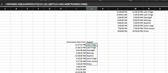
Within a set of time constraints, I am trying to create a formula that will allow me to identify IF a time is between two times, to assign it a text value. I would like to do this for multiple values. The data in M/N/O is the value set for output. Column J is my example of times to use. Column K is my formula entry which has never produced an accurate result. This seems like it should be possible!! What am I missing!! Nothing is working!

Here are a few of the 20+ examples I've tried all day. Initially, I was entering the data in M/N/O by hand, but realized that entering by cell could be easier:

=IF(J4>=$M$2,J4<=$N$2,$O$2),IF(J4>=$M$1,J4<=$N$1,$O$1),IF(J4>=$M$3,J4<=$N$3,$O$3),IF(J4>=$M$4,J4<=$N$4,$O$4),IF(J4>=$M$5,J4<=$N$5,$O$5),IF(J4>=$M$6,J4<=$N$6,$O$6),IF(J4>=$M$7,J4<=$N$7,$O$7)

=IF(J4>$M$2,J4<$N$2,$O$2),IF(J4>$M$1,J4<$N$1,$O$1),IF(J4>$M$3,J4<$N$3,$O$3),IF(J4>$M$4,J4<$N$4,$O$4),IF(J4>$M$5,J4<$N$5,$O$5),IF(J4>$M$6,J4<$N$6,$O$6),IF(J4>$M$7,J4<$N$7,$O$7)

=IF(J4>=$M$2,J4<=$N$2,$O$2),IF(J4>=$M$1,J4<=$N$1,$O$1),IF(J4>=$M$3,J4<=$N$3,$O$3),IF(J4>=$M$4,J4<=$N$4,$O$4),IF(J4>=$M$5,J4<=$N$5,$O$5),IF(J4>=$M$6,J4<=$N$6,$O$6),IF(J4>=$M$7,J4<=$N$7,$O$7)))))))

=IF(AND(J4>=$M$2,J4<$N$2,$O$2),IF(AND(J4>=$M$1,J4<$N$1,$O$1),IF(AND(J4>=$M$3,J4<$N$3,$O$3),IF(AND(J4>=$M$4,J4<$N$4,$O$4),IF(AND(J4>=$M$5,J4<$N$5,$O$5),IF(AND(J4>=$M$6,J4<$N$6,$O$6),IF(AND(J4>=$M$7,J4<$N$7,$O$7)))))))

=IF(AND(J4>=$M$2,J4<$N$2,$O$2),IF(AND(J4>=$M$1,J4<$N$1,$O$1),IF(AND(J4>=$M$3,J4<$N$3,$O$3),IF(AND(J4>=$M$4,J4<$N$4,$O$4),IF(AND(J4>=$M$5,J4<$N$5,$O$5),IF(AND(J4>=$M$6,J4<$N$6,$O$6),IF(AND(J4>=$M$7,J4<$N$7,$O$7))))))))

-- Prior to entering the times in columns, I tried time value as well:
=IF((J5=TIME(20,0,0),J5<=TIME(22,59,59)),”Prime”,IF((J5=TIME(19,0,0),J5<=TIME(19,59,59)),”Prime Access”,IF((J5=TIME(15,0,0),J5<=TIME(18,59,59)),”Early Fringe”, IF((J5=TIME(9,0,0),J5<=TIME(14,59,59)),”Day”, IF((J5=TIME(6,0,0),J5<=TIME(8,59,59)),”Morning”, IF((J5=TIME(2,0,0),J5<=TIME(5,59,59)),”Overnight”, IF((J5=TIME(23,0,0),J5<=TIME(1,59,59)),”Late Fringe”)))))))


I appreciate any assistance. I have 10k+ rows that I will need to enter this for, so the formula creation will be worth days of time.
THANK YOU!

 

[MSWIT310]

OOOOOOOOOH!!! So looking back at my screenshot, I did not in fact know that Peter's formula had to be followed exact - as in, exact order. I DID change the daypart into the two groupings, but paid no attention to the order. That's it! You hit the nail on the head!
So then in fact NOT a PC vs. Mac. Wow. Thank you for helping me to understand! I love this site.

 

[KRice]

See the bottom examples, rows 20:23. The correct answer is "Late Fringe", but if an unsorted table is used with VLOOKUP and the "TRUE" option, this type of error can happen.

mrexcel_20200408.xlsm
	A	B	C	D	E	F	G	H	I	J	K	L	M	N	O
1		1:52:19 PM	Daytime		12:00:00 AM	1:59:59 AM	Late Fringe			1:52:19 PM	Daytime		11:00:00 PM	11:59:59 PM	Late Fringe
2		1:38:33 AM	Late Fringe		2:00:00 AM	5:59:59 AM	Overnight			1:38:33 AM	Late Fringe		12:00:00 AM	1:59:59 AM	Late Fringe
3		6:41:08 PM	Early Fringe		6:00:00 AM	8:59:59 AM	Morning			6:41:08 PM	Early Fringe		2:00:00 AM	5:59:59 AM	Overnight
4		11:48:56 AM	Daytime		9:00:00 AM	2:59:59 PM	Daytime			###########	Daytime		6:00:00 AM	8:59:59 AM	Morning
5		12:47:00 PM	Daytime		3:00:00 PM	6:59:59 PM	Early Fringe			###########	Daytime		9:00:00 AM	2:59:59 PM	Daytime
6		6:39:47 AM	Morning		7:00:00 PM	7:59:59 PM	Prime Access			6:39:47 AM	Morning		3:00:00 PM	6:59:59 PM	Early Fringe
7		8:40:18 AM	Morning		8:00:00 PM	10:59:59 PM	Prime			8:40:18 AM	Morning		7:00:00 PM	7:59:59 PM	Prime Access
8		4:49:07 PM	Early Fringe		11:00:00 PM	12:00:00 AM	Late Fringe			4:49:07 PM	Early Fringe		8:00:00 PM	10:59:59 PM	Prime
9		2:43:34 AM	Overnight							2:43:34 AM	Overnight
10		11:39:11 PM	Late Fringe							###########	Late Fringe
11		1:36:05 AM	Late Fringe							1:36:05 AM	Late Fringe
12		11:36:05 PM	Late Fringe							###########	Late Fringe
13		11:00:00 PM	Late Fringe							###########	Late Fringe
14		12:00:00 AM	Late Fringe							###########	Late Fringe
15		11:59:59 PM	Late Fringe							###########	Late Fringe
16		12:00:01 AM	Late Fringe							###########	Late Fringe
17		10:59:59 PM	Prime							###########	Prime
18
19
20		11:30:00 PM	Prime	Peter's formula with Kirk's lookup table
21		11:30:00 PM	Late Fringe	Peter's formula with Peter's lookup table
22		11:30:00 PM	Late Fringe	Kirk's formula with Kirk's lookup table
23		11:30:00 PM	Late Fringe	Kirk's formula with Peter's lookup table
MSWIT310

Cell Formulas
Range	Formula
C21,C1:C17	C1	=VLOOKUP(B1,E$1:G$8,3)
C23,K1:K17	K1	=INDEX(O$1:O$8,SUMPRODUCT((J1>=M$1:M$8)*(J1<=N$1:N$8)*ROW(O$1:O$8)))
C20	C20	=VLOOKUP(B20,M$1:O$8,3)
C22	C22	=INDEX(O$1:O$8,SUMPRODUCT((B22>=M$1:M$8)*(B22<=N$1:N$8)*ROW(O$1:O$8)))

 

[KRice]

You're welcome...we're glad to help.

 

[MSWIT310]

Hello, I've been using this wonderful formula for 2+ years now, and today, it stopped working. When I paste in the formula "=INDEX(N$1:N$8,SUMPRODUCT((I13>=L$1:L$8)*(I13<=M$1:M$8)*ROW(N$1:N$8)))" it will paste in all the dayparts - not actually using the formula. Do you have ANY idea as to why or how to fix this?

 

[KRice]

I don't see any issue. Could you post a minisheet using XL2BB?...or alternatively, show the formula for one of the cells that is clearly associated with an incorrect result (e.g., 3:17:36 AM should be "Overnight"...what formula appears in your cell such that "Prime Access" is returned?).

MrExcel_20221214.xlsx
	I	J	K	L	M	N
1				11:00:00 PM	11:59:59 PM	Late Fringe
2				12:00:00 AM	1:59:59 AM	Late Fringe
3				2:00:00 AM	5:59:59 AM	Overnight
4				6:00:00 AM	8:59:59 AM	Morning
5				9:00:00 AM	2:59:59 PM	Daytime
6				3:00:00 PM	6:59:59 PM	Early Fringe
7				7:00:00 PM	7:59:59 PM	Prime Access
8				8:00:00 PM	10:59:59 PM	Prime
9
10
11
12	Occurrence Start Time	Daypart
13	11:27:53 PM	Late Fringe
14	11:56:13 PM	Late Fringe
15	4:55:48 AM	Overnight
16	6:38:45 PM	Early Fringe
17	12:58:38 AM	Late Fringe
18	6:45:05 PM	Early Fringe
19	3:17:36 AM	Overnight
20	3:33:30 PM	Early Fringe
21	3:36:53 PM	Early Fringe
22	9:12:59 AM	Daytime
23	12:22:26 PM	Daytime
MSWIT310_20221213

Cell Formulas
Range	Formula
J13:J23	J13	=INDEX(N$1:N$8,SUMPRODUCT((I13>=L$1:L$8)*(I13<=M$1:M$8)*ROW(N$1:N$8)))

 

[Peter_SSs]

Do you have ANY idea as to why or how to fix this?

It looks to me like two things could be involved here (though remember that I do not have a mac to check)

1. The fact that those values automatically 'spilled' down the column indicated that your profile may no longer be correct (unless Excel 2019 now 'spills' results?)
   
   
2. That behaviour would occur (in Excel 365 for example) if some of the times are actual times (numbers) and some of the times are text. In the sample below, all the times in columns L & M are actual times (numerical) but you see different results in the bottom section depending on whether those times ate numerical or not. With the formula in H13, because the 'time' is actually text, the formula is not finding that 'time' between any of the column L & M values (text values are always > numerical values in Excel) so the SUMPRODUCT is returning 0. When you index a column with the value 0, it returns the whole column, which is what has happened in column H

22 12 14.xlsm
	G	H	I	J	K	L	M	N
1						11:00:00 PM	11:59:59 PM	Late Fringe
2						12:00:01 AM	1:59:59 AM	Late Fringe
3						2:00:00 AM	5:59:59 AM	Overnight
4						6:00:00 AM	8:59:59 AM	Morning
5						9:00:00 AM	2:59:59 PM	Raytime
6						3:00:00 PM	6:59:59 PM	Early Fringe
7						7:00:00 PM	7:59:59 PM	Prime Access
8						8:00:00 PM	10:59:59 PM	Prime Access
9
10
11
12	FALSE		TRUE
13	11:27:53 PM	Late Fringe	11:27:53 PM	Late Fringe
14		Late Fringe
15		Overnight
16		Morning
17		Raytime
18		Early Fringe
19		Prime Access
20		Prime Access
21
Test

Cell Formulas
Range	Formula
G12,I12	G12	=ISNUMBER(G13)
H13:H20	H13	=INDEX(N$1:N$8,SUMPRODUCT((G13>=L$1:L$8)*(G13<=M$1:M$8)*ROW(N$1:N$8)))
J13	J13	=INDEX(N$1:N$8,SUMPRODUCT((I13>=L$1:L$8)*(I13<=M$1:M$8)*ROW(N$1:N$8)))
Dynamic array formulas.