If = to 20 Then Paste Formula in Cell Loop

[ChrisOK]

Was trying to do with a small lookup table (If = 20, then go find 20 in Col N and paste formula found inadjacent cell of Col O) but gave up on that route..
Found the BELOW might be a better/hard coded way to do it -- just not sure how to change the "Interior.Color" action to a Paste this formula INSTEAD action..

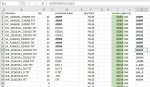
• Col A has varied filenames with diff lengths..
• Col B has a LEN formula in it that provides the length (anywhere from 14 to 22 so far)
• Col K is where I want to paste a formula that will be specific if the LEN is 14, a different formula if the LEN is 15, etc)

Example:........ IF oCell (which would be B2) = "14" Then PASTE THIS FORMULA into adjacent Col K =MID(B2,6,5)
............................ELSE...........see if that cell is = to "15".................if this is true, paste a different formula... =MID(B2,7,5)
............................ELSE...........see if it's = to ..............."16".................if this is true, paste a different formula... =MID(B2,8,5)
............................ELSE...........see if it's = to ..............."17".................if this is true, paste a different formula... =MID(B2,9,5)
............................ELSE...........see if it's = to ..............."18".................if this is true, paste a different formula... =MID(B2,10,5)
............................ELSE...........see if it's = to ..............."19".................if this is true, paste a different formula... =MID(B2,11,5)
............................ELSE...........see if it's = to ..............."20".................if this is true, paste a different formula... =MID(B2,12,5)
............................ELSE...........see if it's = to ..............."21".................if this is true, paste a different formula... =MID(B2,13,5)
............................ELSE...........see if it's = to ..............."22".................if this is true, paste a different formula... =MID(B2,14,5)
Once it finds a match and pastes it's appropriate formula to use, move to next cell... and adjust formula cell reference to be adjacent
In other words, I need to use B2 in the formula IF on row 2, .......use B3 within the formula if on row 3
I don't want a formula that looks like this to happen on row 10 (B10): =MID(B2,5,6)
Instead the formula on row 10 (B10) should look like this: ......................... =MID(B10,5,6)

....(next cell).....IF oCell (which would be B3) = "21" Then PASTE THIS FORMULA into adjacent Col K =MID(B3,13,5)

Here's what I thought might work well but not sure how to adjust it to paste various formulas instead of colorizing)

Sub Range_LoopCells()

Dim oRange As Range
Dim oCell As Range

Set oRange = Sheets(1).Range("B2:B365")

For Each oCell In oRange
    If oCell = "14" Then oCell.Interior.Color = vbRed
    If oCell = "15" Then oCell.Interior.Color = vbGreen
    If oCell = "16" Then oCell.Interior.Color = vbYellow
    If oCell = "17" Then oCell.Interior.Color = vbGreen
    If oCell = "18" Then oCell.Interior.Color = vbRed
    If oCell = "19" Then oCell.Interior.Color = vbGreen
    If oCell = "20" Then oCell.Interior.Color = vbGreen
    If oCell = "21" Then oCell.Interior.Color = vbGreen
    If oCell = "22" Then oCell.Interior.Color = vbRed
Next oCell

End Sub

Thank you in advance!

 

[DanteAmor]

Example:........ IF oCell (which would be B2) = "14" Then PASTE THIS FORMULA into adjacent Col K =MID(B2,6,5)

But what is the final objective, that is, you want to extract a data from cell A.
You could put examples of the data you have in column A and what is the result you want.
What I want to know is what result you want in column K, that way you can simplify your macro, and maybe you don't need the length you have in column B.

 

[DanteAmor]

Check if the following results in column K are what you need.

Sub NewFormula()
  With Range("K2:K" & Range("A" & Rows.Count).End(3).Row)
    .Formula = "=LEFT(RIGHT(A2,9),5)"
  End With
End Sub

If you only want the values then try the following:

Sub NewFormula()
  With Range("K2:K" & Range("A" & Rows.Count).End(3).Row)
    .Formula = "=LEFT(RIGHT(A2,9),5)"
    .Value = .Value
  End With
End Sub

 

[ChrisOK]

VBA Code:
Sub NewFormula()
With Range("K2:K" & Range("A" & Rows.Count).End(3).Row)
.Formula = "=LEFT(RIGHT(A2,9),5)"
End With
End Sub

@DanteAmor:
The first one above pastes a formula, but the problem is, I do not want the same formula pasted all the way down as each filename found in Col A has varied lengths.
So, to answer your orig question: (result formula should YES be pasted into Col K)
I was using Col B (which denotes the LEN result) to determine which formula should be pasted into K

• If LEN is x then paste this formula
• If LEN is y then paste this formula
• If LEN is z then paste this formula
• If nothing, then skip cell and continue until no more data exists in Col B to evaluate)

In the attached image, I've struck through all the ones in Col K that are not acceptable - it's bc the same formula can't work for every LEN
Also, YES, the Col B could be eliminated if the formula/lookup can be a combined command that (1) determines LEN of A, then uses the formula that corresponds with that designated LEN parameter)
*Another thing to note, the format of Col A filenames varies -- they won't always have an underscore.. diff mainframe filenames w/ varied formats (but the rules examples in my orig post will always work based on the same formats that will appear in Col A)

 

[DanteAmor]

Let's forget the formulas and macros.
Put here the different examples of file names that you could have and what is the data that you require of each one of them.
It also explains if there is any pattern in the names of the files to obtain the data that you need. (In addition to length.)
Also put the examples with XL2BB tool since from the image I cannot copy them.

 

[ChrisOK]

The examples will vary and I don't yet know what could still-yet be coming down the pipe - can't give you exact file formats.
End goal is to extract the Julian dates from the filenames in Col A and placed into Col K so they can be batched & dumped into designated system folders.
The "known" requirements that I know will work are the following:
IF B2 = "14" Then =MID(B2,6,5)
IF B2 = "15" Then =MID(B2,7,5)
IF B2 = "16" Then =MID(B2,8,5)
IF B2 = "17" Then =MID(B2,9,5)
IF B2 = "18" Then =MID(B2,10,5)
IF B2 = "19" Then =MID(B2,11,5)
IF B2 = "20" Then =MID(B2,12,5)
IF B2 = "21" Then =MID(B2,13,5)
IF B2 = "22" Then =MID(B2,14,5)
ELSE NOTHING (leave blank)

Alternatively, Col B could be eliminated, IF the formula or vba combined the LEN eval with the pasting of the designated formula
Example:
IF A2 LEN is "14" Then =MID(B2,6,5) gets placed into K2

On a work laptop that won't allow the other add-in tool, but the above shortened version should be copy/pasteable for more ease.

 

[DanteAmor]

There is some pattern in the names.
According to your examples: all the acceptable ones have an underscore "_"
Or maybe it can be the letter D followed by 5 digits
Or maybe 5 digits and ".txt"
If you comment which one or what the patterns are then you can get the number, and those that do not meet the patterns the result are empty.

______________________________________________________________________________

The "known" requirements that I know will work are the following:

But if you insist on only considering names with a length between 14 and 22, but considering only numbers, Try this:

Sub NewFormula()
  With Range("K2:K" & Range("A" & Rows.Count).End(3).Row)
    .Formula = "=IF(AND(LEN(A2)>=14,LEN(A2)<=22),IF(ISNUMBER(--LEFT(RIGHT(A2,9),5)),LEFT(RIGHT(A2,9),5),""""),"""")"
    .Value = .Value
  End With
End Sub

 

[NoSparks]

Use BobBridges suggestion at MSOfficeForums of making the formulas in your lookup table like this with the leading single quote
'=MID(ZZ,6,5)
the NOTHING isn't required in your table

Then use this macro to insert the formula into column "K"

Sub InsertingForumlas()
    Dim ws As Worksheet, rng As Range, cel As Range, x As Long
    Dim fndLngth As Range, ThisFormula As String
    
Set ws = Sheets("51batchWmoreScenarios")

With ws
    Set rng = .Range("A2", .Range("A" & Rows.Count).End(xlUp))
    For Each cel In rng
        x = Len(cel.Value)
        Set fndLngth = .Range("N:N").Find(x, , xlValues, xlWhole, xlByRows, xlNext, False)
        If Not fndLngth Is Nothing Then
            cel.Offset(, 10) = Replace(fndLngth.Offset(, 1), "ZZ", "A" & cel.Row)
        Else
            cel.Offset(, 10) = "NOTHING"
        End If
    Next cel
End With

End Sub

Your post 7 over there included 4 file names of 24 characters, me thinks the formula for those will be interesting.

 

[Fluff]

Cross posted PASTE FORMULA from lookup table

While we do allow Cross-Posting on this site, we do ask that you please mention you are doing so and provide links in each of the threads pointing to the other thread (see rule 13 here along with the explanation: Forum Rules). This way, other members can see what has already been done in regards to a question, and do not waste time working on a question that may already be answered.