Index product based on Location + sum

[anoop0085]

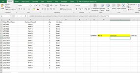
Guy below you can see i have excel sheet (2016) were i am posting day to day purchases . Each it kept in a particular location/ boxes on each posting. Now i need a formula to index all items(cell no I8 to below) which in particular a box (cell no h7) with total qty purchased in that box . Hope you understand and help me with the formula

Test store.xlsx
	A	B	C	D	E	F	G	H	I	J	K
1	Date of Purchase	Item purchased	qty	Location
2	5/4/2022	Item A	2	Box 1
3	5/5/2022	Item B	1	Box 2
4	5/6/2022	Item C	1	Box 2
5	5/7/2022	Item B	2	Box 1
6	5/8/2022	Item D	1	Box 3
7	5/9/2022	Item A	2	Box 4			Location :	Box 1	Item List	Total qty
8	5/10/2022	Item E	1	Box 1					?	?
9	5/11/2022	Item E	1	Box 3					?	?
10	5/12/2022	Item D	3	Box 4					?	?
11	5/13/2022	Item C	1	Box 1					?	?
12	5/14/2022	Item B	5	Box 1					?	?
13	5/15/2022	Item D	1	Box 2					?	?
14	5/16/2022	Item A	1	Box 2					?	?
15	5/17/2022	Item E	2	Box 3					?	?
16	5/18/2022	Item B	6	Box 4					?	?
17	5/19/2022	Item D	1	Box 1					?	?
18	5/20/2022	Item C	1	Box 2					?	?
19	5/21/2022	Item B	4	Box 4					?	?
20	5/22/2022	Item D	1	Box 3					?	?
21									?	?
22
Sheet1

Cells with Data Validation
Cell	Allow	Criteria
H7	List	=$M$2:$M$5

 

[Mposwal]

Use formulas as below:

I8 => =SORT(UNIQUE(FILTER(B2:B19,D2:D19=H7)))
J8=> =SUMIFS($C$2:$C$19,$B$2:$B$19,I8,$D$2:$D$19,$H$7)

 

[Mposwal]

 

[Peter_SSs]

@Mposwal
If you look at what is written in post #1 and at the OP's details in the left hand column you will see that they are using Excel 2016 so will not have access to some of the functions that you are suggesting.

@anoop0085
Can you post another mini-sheet with the expected results manually filled in?

 

[anoop0085]

@Mposwal
If you look at what is written in post #1 and at the OP's details in the left hand column you will see that they are using Excel 2016 so will not have access to some of the functions that you are suggesting.

@anoop0085
Can you post another mini-sheet with the expected results manually filled in?

Test store.xlsx
	A	B	C	D	E	F	G	H	I	J
1	Date of Purchase	Item purchased	qty	Location
2	5/4/2022	Item A	2	Box 1
3	5/5/2022	Item B	1	Box 2
4	5/6/2022	Item C	1	Box 2
5	5/7/2022	Item B	2	Box 1
6	5/8/2022	Item D	1	Box 3
7	5/9/2022	Item A	2	Box 4			Location :	Box 1	Item List	Total qty
8	5/10/2022	Item E	1	Box 1					Item A	2
9	5/11/2022	Item E	1	Box 3					Item B	2+5=7
10	5/12/2022	Item D	3	Box 4					Item E	1
11	5/13/2022	Item C	1	Box 1					Item C	1
12	5/14/2022	Item B	5	Box 1					Item D	1
13	5/15/2022	Item D	1	Box 2					?	?
14	5/16/2022	Item A	1	Box 2					?	?
15	5/17/2022	Item E	2	Box 3					?	?
16	5/18/2022	Item B	6	Box 4					?	?
17	5/19/2022	Item D	1	Box 1					?	?
18	5/20/2022	Item C	1	Box 2					?	?
19	5/21/2022	Item B	4	Box 4					?	?
20	5/22/2022	Item D	1	Box 3
21
22
Sheet1

Cells with Data Validation
Cell	Allow	Criteria
H7	List	=$M$2:$M$5

 

[Peter_SSs]

Thanks for the additional information. Try this.

22 08 04.xlsm
	A	B	C	D	E	F	G	H	I	J
1	Date of Purchase	Item purchased	qty	Location
2	5/04/2022	Item A	2	Box 1
3	5/05/2022	Item B	1	Box 2
4	5/06/2022	Item C	1	Box 2
5	5/07/2022	Item B	2	Box 1
6	5/08/2022	Item D	1	Box 3
7	5/09/2022	Item A	2	Box 4			Location :	Box 1	Item List	Total qty
8	5/10/2022	Item E	1	Box 1					Item A	2
9	5/11/2022	Item E	1	Box 3					Item B	7
10	5/12/2022	Item D	3	Box 4					Item E	1
11	5/13/2022	Item C	1	Box 1					Item C	1
12	5/14/2022	Item B	5	Box 1					Item D	1
13	5/15/2022	Item D	1	Box 2
14	5/16/2022	Item A	1	Box 2
15	5/17/2022	Item E	2	Box 3
16	5/18/2022	Item B	6	Box 4
17	5/19/2022	Item D	1	Box 1
18	5/20/2022	Item C	1	Box 2
19	5/21/2022	Item B	4	Box 4
20	5/22/2022	Item D	1	Box 3
Qty

Cell Formulas
Range	Formula
I8:I20	I8	=IFERROR(INDEX(B:B,AGGREGATE(15,6,ROW(B$2:B$20)/((D$2:D$20=H$7)*ISNA(MATCH(B$2:B$20,I$7:I7,0))),1)),"")
J8:J20	J8	=IF(I8="","",SUMIFS(C$2:C$20,B$2:B$20,I8,D$2:D$20,H$7))

 

[anoop0085]

Thanks for the additional information. Try this.

22 08 04.xlsm
	A	B	C	D	E	F	G	H	I	J
1	Date of Purchase	Item purchased	qty	Location
2	5/04/2022	Item A	2	Box 1
3	5/05/2022	Item B	1	Box 2
4	5/06/2022	Item C	1	Box 2
5	5/07/2022	Item B	2	Box 1
6	5/08/2022	Item D	1	Box 3
7	5/09/2022	Item A	2	Box 4			Location :	Box 1	Item List	Total qty
8	5/10/2022	Item E	1	Box 1					Item A	2
9	5/11/2022	Item E	1	Box 3					Item B	7
10	5/12/2022	Item D	3	Box 4					Item E	1
11	5/13/2022	Item C	1	Box 1					Item C	1
12	5/14/2022	Item B	5	Box 1					Item D	1
13	5/15/2022	Item D	1	Box 2
14	5/16/2022	Item A	1	Box 2
15	5/17/2022	Item E	2	Box 3
16	5/18/2022	Item B	6	Box 4
17	5/19/2022	Item D	1	Box 1
18	5/20/2022	Item C	1	Box 2
19	5/21/2022	Item B	4	Box 4
20	5/22/2022	Item D	1	Box 3
Qty

Cell Formulas
Range	Formula
I8:I20	I8	=IFERROR(INDEX(B:B,AGGREGATE(15,6,ROW(B$2:B$20)/((D$2:D$20=H$7)*ISNA(MATCH(B$2:B$20,I$7:I7,0))),1)),"")
J8:J20	J8	=IF(I8="","",SUMIFS(C$2:C$20,B$2:B$20,I8,D$2:D$20,H$7))

Your formula is working but some reason when i click box 1 nothing is showing , any suggestion ?- other is working

 

[anoop0085]

Your formula is working but some reason when i click box 1 nothing is showing , any suggestion ?- other is working

sorry for mis understanding , it think it is issue with text , thank you all specially @Peter_SSs

 

[Peter_SSs]

Everything working okay now?
I notice that it looks like you have entered the formula as an array formula (Ctrl+Shift+Enter). I don't think that you should need to do that.

 

[anoop0085]

ok , it just did that because box 1 did not work first time