Is it possible to use IF and Vlookup?

harriet60

New Member
Joined
Apr 6, 2022
Messages
18
Office Version
  1. 365
Platform
  1. Windows
Hello everyone
Hoping someone can help again please!
I am trying to use IF and Vlookup together but can't get it to work.
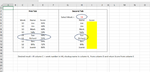
I have one sheet of data that has results by week (column A = week, column B = Name, Column C = Score Achieved
I then have a second sheet that has column A = Name, column B = Score Achieved, and a single cell with a week number in it (also validated to a list so week number can be changed)
What I am trying to achieve is - If week number is = to single cell number ie: 11, vlookup the name and return the score achieved. Thus, whenever the week number is changed, the vlookup will return the correct data for the week selected.
As always, thanks in advance for any help anyone can give.
 

Attachments

  • IF VLOOKUP.png
    IF VLOOKUP.png
    39 KB · Views: 16

Excel Facts

When did Power Query debut in Excel?
Although it was an add-in in Excel 2010 & Excel 2013, Power Query became a part of Excel in 2016, in Data, Get & Transform Data.
Try XLOOKUP.
Book1.xlsx
ABCDEFGHI
1
2
3
411
5WeekNameScore
610Joe95%Joe 
710Jim40%Jim
810Mark60%Mark
910Sally59%Sally
1011Sue99%Sue99%
1111Richard55%Richard55%
1212Ben69%Ben
1312Billy72%Billy
1412Joanie86%Joanie
Sheet8
Cell Formulas
RangeFormula
I6:I14I6=XLOOKUP(H4&H6:H14,C6:C14&D6:D14,E6:E14,"")
Dynamic array formulas.
 
Upvote 0
Try:
Book1
ABCDEFGHI
1First TabSecond Tab
2Select Week >11
3WeekNameScoreNameScore
410Joe95%Joe 
510Jim40%Jim 
610Mark60%Mark 
710Sally59%Sally 
811Sue99%Sue99%
911Richard55%Richard55%
1012Ben69%Ben 
1112Billy72%Billy 
1212Joanie86%Joanie 
Sheet1
Cell Formulas
RangeFormula
I4:I12I4=FILTER($C$4:$C$12,($B$4:$B$12=H4)*($A$4:$A$12=$H$2),"")
 
Upvote 0
Solution
so in your example
i would use index match , but vlookup should work

=index($E$6:$E$14, match($H$4&H6, $C$6:$C$14&$D$6:$D$14,0))
=IFERROR(index($E$6:$E$14, match($H$4&H6, $C$6:$C$14&$D$6:$D$14,0)),"")


Book1
ABCDEFGHI
1
2
3
411
5WeekNameScore
610Joe0.95Joe 
710Jim0.4Jim 
810Mark0.6Mark 
910Sally0.59Sally 
1011Sue0.99Sue0.99
1111Richard0.55Richard0.55
1212Ben0.69Ben 
1312Billy0.72Billy 
1412Joanie0.86Joanie 
Sheet1
Cell Formulas
RangeFormula
I6:I14I6=IFERROR(INDEX($E$6:$E$14, MATCH($H$4&H6, $C$6:$C$14&$D$6:$D$14,0)),"")
 
Upvote 0
Try XLOOKUP.
Book1.xlsx
ABCDEFGHI
1
2
3
411
5WeekNameScore
610Joe95%Joe 
710Jim40%Jim
810Mark60%Mark
910Sally59%Sally
1011Sue99%Sue99%
1111Richard55%Richard55%
1212Ben69%Ben
1312Billy72%Billy
1412Joanie86%Joanie
Sheet8
Cell Formulas
RangeFormula
I6:I14I6=XLOOKUP(H4&H6:H14,C6:C14&D6:D14,E6:E14,"")
Dynamic array formulas.
Thankyou for your help - it works beautifully :)
 
Upvote 0
Try:
Book1
ABCDEFGHI
1First TabSecond Tab
2Select Week >11
3WeekNameScoreNameScore
410Joe95%Joe 
510Jim40%Jim 
610Mark60%Mark 
710Sally59%Sally 
811Sue99%Sue99%
911Richard55%Richard55%
1012Ben69%Ben 
1112Billy72%Billy 
1212Joanie86%Joanie 
Sheet1
Cell Formulas
RangeFormula
I4:I12I4=FILTER($C$4:$C$12,($B$4:$B$12=H4)*($A$4:$A$12=$H$2),"")
Thankyou also for your help = this too works beautifully :)
 
Upvote 0
so in your example
i would use index match , but vlookup should work

=index($E$6:$E$14, match($H$4&H6, $C$6:$C$14&$D$6:$D$14,0))
=IFERROR(index($E$6:$E$14, match($H$4&H6, $C$6:$C$14&$D$6:$D$14,0)),"")


Book1
ABCDEFGHI
1
2
3
411
5WeekNameScore
610Joe0.95Joe 
710Jim0.4Jim 
810Mark0.6Mark 
910Sally0.59Sally 
1011Sue0.99Sue0.99
1111Richard0.55Richard0.55
1212Ben0.69Ben 
1312Billy0.72Billy 
1412Joanie0.86Joanie 
Sheet1
Cell Formulas
RangeFormula
I6:I14I6=IFERROR(INDEX($E$6:$E$14, MATCH($H$4&H6, $C$6:$C$14&$D$6:$D$14,0)),"")
Thank you also for your help - this formula also works beautifully :)
 
Upvote 0

Forum statistics

Threads
1,216,783
Messages
6,132,678
Members
449,747
Latest member
OldMrsMol

We've detected that you are using an adblocker.

We have a great community of people providing Excel help here, but the hosting costs are enormous. You can help keep this site running by allowing ads on MrExcel.com.
Allow Ads at MrExcel

Which adblocker are you using?

Disable AdBlock

Follow these easy steps to disable AdBlock

1)Click on the icon in the browser’s toolbar.
2)Click on the icon in the browser’s toolbar.
2)Click on the "Pause on this site" option.
Go back

Disable AdBlock Plus

Follow these easy steps to disable AdBlock Plus

1)Click on the icon in the browser’s toolbar.
2)Click on the toggle to disable it for "mrexcel.com".
Go back

Disable uBlock Origin

Follow these easy steps to disable uBlock Origin

1)Click on the icon in the browser’s toolbar.
2)Click on the "Power" button.
3)Click on the "Refresh" button.
Go back

Disable uBlock

Follow these easy steps to disable uBlock

1)Click on the icon in the browser’s toolbar.
2)Click on the "Power" button.
3)Click on the "Refresh" button.
Go back
Back
Top