JenniferMurphy
Well-known Member
- Joined
- Jul 23, 2011
- Messages
- 2,533
- Office Version
- 365
- Platform
- Windows
Please bear with my rather long and involved intro. The question is at the end.
In my effort to convert Amazon-type ratings to meaningful z scores, I came up with the table below. Columns F-J are used to calculate columns L-P, which are used to calculate the mean and std dev, which are used to calculate the confidence intervals, which are used to adjust the ratings, which can then be converted to z scores.
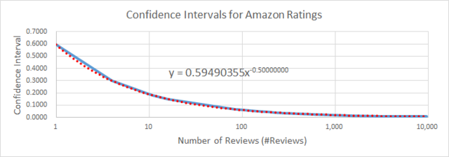
To see whether there is a reliable relationship between the number of reviews and the confidence intervals, I plotted them in a scatter chart and added a trendline. It turns out that a power equation is a near perfect fit. I don't see a way to post a chart using xl2bb, so here it is as a graphic.
 I then use that
I then used that equation to compute a confidence interval directly from the number of reviews. There is very little difference. This allows me to bypass all of the other math above and calculate adjusted ratings directly from the number of reviews.
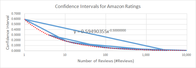
Here's the problem. I would like to be able to sort the table in several ways, but if I do, the chart gets all screwed up. Here's what happens if I sort the table on the Rank1 field.

Or if I sort it on the SKU column.
Is there any way that I can set it up so that I can sort the table anyway I want without affecting the chart?
I do not want to freeze the chart, unless there is also a way to unfreeze it, as I may want to add additional rows to the table and have te chart and trendline updated.
Thanks. I hope this was not too muddled.
In my effort to convert Amazon-type ratings to meaningful z scores, I came up with the table below. Columns F-J are used to calculate columns L-P, which are used to calculate the mean and std dev, which are used to calculate the confidence intervals, which are used to adjust the ratings, which can then be converted to z scores.
| Cell Formulas | ||
|---|---|---|
| Range | Formula | |
| L5:L20 | L5 | =[@['#Reviews]]*[@[5%]] |
| M5:M20 | M5 | =[@['#Reviews]]*[@[4%]] |
| N5:N20 | N5 | =[@['#Reviews]]*[@[3%]] |
| O5:O20 | O5 | =[@['#Reviews]]*[@[2%]] |
| P5:P20 | P5 | =[@['#Reviews]]*[@[1%]] |
| Q5:Q20 | Q5 | =SUM([@['#5]]:[@['#1]]*{5,4,3,2,1})/[@['#Reviews]] |
| R5:R20 | R5 | =SQRT(SUM(({5,4,3,2,1}-[@Mean])^2*[@['#5]]:[@['#1]])/[@['#Reviews]]) |
| S5:S20 | S5 | =CONFIDENCE.NORM(Alpha,TblAmz3[[#Totals],[Std Dev]],[@['#Reviews]]) |
| L21 | L21 | =SUBTOTAL(101,['#5]) |
| M21 | M21 | =SUBTOTAL(101,['#4]) |
| N21 | N21 | =SUBTOTAL(101,['#3]) |
| O21 | O21 | =SUBTOTAL(101,['#2]) |
| P21 | P21 | =SUBTOTAL(101,['#1]) |
| Q21 | Q21 | =SUBTOTAL(101,[Mean]) |
| R21 | R21 | =SUBTOTAL(101,[Std Dev]) |
| S21 | S21 | =SUBTOTAL(101,[Conf Int]) |
| U5:U20 | U5 | =RANK.EQ([@[Rtg Adj]],[Rtg Adj]) |
| V5:V20 | V5 | =[@Rtg]-[@[Rtg Adj]] |
| W5:W20 | W5 | =[@Rank1]-[@Rank2] |
| E5:E20 | E5 | =RANK([@Rtg],[Rtg])+SUMPRODUCT(--([Rtg]=[@Rtg]),--([@['#Reviews]]<['#Reviews])) |
| K5:K20 | K5 | =SUM([@[5%]]:[@[1%]]) |
| Y5:Y20 | Y5 | =([@[Conf Int2]]/[@[Conf Int]])-1 |
| C21 | C21 | =SUBTOTAL(101,[Rtg]) |
| D21 | D21 | =SUBTOTAL(101,['#Reviews]) |
| F21 | F21 | =SUBTOTAL(101,[5%]) |
| G21 | G21 | =SUBTOTAL(101,[4%]) |
| H21 | H21 | =SUBTOTAL(101,[3%]) |
| I21 | I21 | =SUBTOTAL(101,[2%]) |
| J21 | J21 | =SUBTOTAL(101,[1%]) |
| X5:X20 | X5 | =Coef * ([@['#Reviews]]^Expon) |
| X21 | X21 | =SUBTOTAL(101,[Conf Int2]) |
| T5:T20 | T5 | =[@Rtg]-[@[Conf Int]] |
| T21 | T21 | =SUBTOTAL(101,[Rtg Adj]) |
| T22 | T22 | =STDEV.S(TblAmz3[Rtg Adj]) |
| Z5:Z20 | Z5 | =([@[Rtg Adj]]-TblAmz3[[#Totals],[Rtg Adj]])/RtgAdjStdDev |
| Z21 | Z21 | =SUBTOTAL(101,[RtgZ]) |
| Z22 | Z22 | =STDEV.S(TblAmz3[RtgZ]) |
| Named Ranges | ||
|---|---|---|
| Name | Refers To | Cells |
| 'Chart & Sort'!Alpha | ='Chart & Sort'!$S$2 | S5:S20 |
| 'Chart & Sort'!Coef | ='Chart & Sort'!$X$2 | X5:X20 |
| 'Chart & Sort'!Expon | ='Chart & Sort'!$X$3 | X5:X20 |
| 'Chart & Sort'!RtgAdjStdDev | ='Chart & Sort'!$T$22 | Z5:Z20 |
To see whether there is a reliable relationship between the number of reviews and the confidence intervals, I plotted them in a scatter chart and added a trendline. It turns out that a power equation is a near perfect fit. I don't see a way to post a chart using xl2bb, so here it is as a graphic.
I then used that equation to compute a confidence interval directly from the number of reviews. There is very little difference. This allows me to bypass all of the other math above and calculate adjusted ratings directly from the number of reviews.
Here's the problem. I would like to be able to sort the table in several ways, but if I do, the chart gets all screwed up. Here's what happens if I sort the table on the Rank1 field.
Or if I sort it on the SKU column.
Is there any way that I can set it up so that I can sort the table anyway I want without affecting the chart?
I do not want to freeze the chart, unless there is also a way to unfreeze it, as I may want to add additional rows to the table and have te chart and trendline updated.
Thanks. I hope this was not too muddled.


