I have a VBA script that I would like to add some total funtions to. It was originally done by a third party and also is in spanish. I speak neither spanish or VBA. If my terminology or anything is terrible please be patient with me as I dont do much coding. I typically make minor alterations to existing code to better suit my needs. I've been able to get it to add new column titles and the information but figuring out how to total it up has me lost.
A short description of the code is that I open the sheet with the Macro in it. Run the macro which asks me to find the sheet I'm working with and then it goes down column A and finds the block name and then copies information from a database into that row. After doing that for all of the blocks then it will organize them by color.
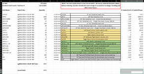
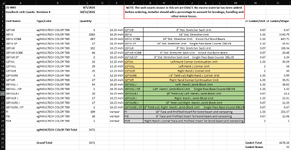
The number/location/Order of the columns will always stay the same but the number of rows will always be different. One constant is that at the very bottom of the sheet in column B will always be "Grand Total". My thought was to script a way at the end to find the cell with "Grand Total", move 12 cells over to column N, Input "Gasket Total" (in bold, and resize column to fit text), move one cell over and input a formula giving a total for column O. Then move one row down, one column left and input "Gasket Boxes" (in bold). Move one cell over and take the gasket total, divide by 200, and round up to the nearest whole number. The end goal just being that the total quantity of gasket material is listed along with how many boxes that ends up being rounded up.
Attached are two images. One showing how the code completes currently and one showing what I'm trying to achieve.
Attached is most of the code. Its at least the part i've been modifying to add the new gasket columns. If theres any questions about it I can do my best to answer but I did not write it nor do I know much about VBA. Please let me know if I need to provide any additional sheets (like the database), sample sheet, ect. If you provide just the additional code please also tell me where I would need to insert the code for it to function. I literally have a day at best of working with VBA and it gets over my head quickly.
Thank you all very much.
A short description of the code is that I open the sheet with the Macro in it. Run the macro which asks me to find the sheet I'm working with and then it goes down column A and finds the block name and then copies information from a database into that row. After doing that for all of the blocks then it will organize them by color.
The number/location/Order of the columns will always stay the same but the number of rows will always be different. One constant is that at the very bottom of the sheet in column B will always be "Grand Total". My thought was to script a way at the end to find the cell with "Grand Total", move 12 cells over to column N, Input "Gasket Total" (in bold, and resize column to fit text), move one cell over and input a formula giving a total for column O. Then move one row down, one column left and input "Gasket Boxes" (in bold). Move one cell over and take the gasket total, divide by 200, and round up to the nearest whole number. The end goal just being that the total quantity of gasket material is listed along with how many boxes that ends up being rounded up.
Attached are two images. One showing how the code completes currently and one showing what I'm trying to achieve.
Attached is most of the code. Its at least the part i've been modifying to add the new gasket columns. If theres any questions about it I can do my best to answer but I did not write it nor do I know much about VBA. Please let me know if I need to provide any additional sheets (like the database), sample sheet, ect. If you provide just the additional code please also tell me where I would need to insert the code for it to function. I literally have a day at best of working with VBA and it gets over my head quickly.
VBA Code:
Private Sub CommandButton1_Click()
'
' Import
'
' BOTON PARA CARGAR LOS DATOS EN EL ACTUAL LIBRO PROVENIENTES DE OTROS LIBROS EXTERNOS
Application.ScreenUpdating = False
Application.DisplayAlerts = False
Dim WorkBookOrigen, WorkbookDestino As Workbook
Dim HojaOrigen As Excel.Worksheet, _
    HojaDestino As Excel.Worksheet, _
    RutaO As String
Dim i, j, ColoNum, BF, BI, r As Integer
Dim HojaMain As Excel.Worksheet, _
    HojaInsultechColorations As Excel.Worksheet

Sheets("InsultechColorations").Visible = True
'############################################
' Aquí se coloca la información que se
' almacena en "18-0070"
'############################################

'Se reconoce el libro destino como el actual
Set WorkbookDestino = ActiveWorkbook

' Se limpia el contenido previo
Sheets("Main").Select
Cells.Delete 'o ClearContents
Range("A1").Select
RutaO = ActiveWorkbook.Path & "\" & ComboBox1.Value
Set WorkBookOrigen = Workbooks.Open(RutaO)

WorkBookOrigen.Worksheets(1).Range("A:AZ").Copy

' Se exporta el contenido de la Base de datos
Set HojaDestino = WorkbookDestino.Worksheets("Main")

WorkbookDestino.Activate
HojaDestino.Select
HojaDestino.Range("A1").Select
ActiveSheet.Paste
Range("A2").Select
ActiveCell.FormulaR1C1 = "Insultech Unit Counts"

Range("N4").Select
ActiveCell.FormulaR1C1 = "LF Gasket/Unit"
Range("O4").Select
ActiveCell.FormulaR1C1 = "LF Gasket/Shape"

Columns("A:O").EntireColumn.AutoFit
Rows("1:5").Select
Selection.Font.Bold = True

WorkBookOrigen.Save
WorkBookOrigen.Close
Range("A1").Select


'############################################
' Aquí se coloca la información que se
' almacena "InsultechColorations"
'############################################

' Se limpia el contenido previo
Sheets("InsultechColorations").Select
Cells.Delete
Range("A1").Select
RutaO = ActiveWorkbook.Path & "\" & "InsultechColorations"
Set WorkBookOrigen = Workbooks.Open(RutaO)

WorkBookOrigen.Worksheets(1).Range("A:AZ").Copy

' Se exporta el contenido de la Base de datos
Set HojaDestino = WorkbookDestino.Worksheets("InsultechColorations")

WorkbookDestino.Activate
HojaDestino.Select
HojaDestino.Range("A1").Select
Selection.PasteSpecial Paste:=xlPasteAllUsingSourceTheme, Operation:=xlNone _
    , SkipBlanks:=False, Transpose:=False

Sheets("InsultechColorations").Select
Range("L2:S4").Select
Selection.Copy
Sheets("Main").Select
Range("F1").Select
ActiveSheet.Paste

WorkBookOrigen.Save
WorkBookOrigen.Close

'##############################################
'############ Coincide y copia ################
'##############################################

Set HojaMain = ActiveWorkbook.Worksheets("Main")

Set HojaInsultechColorations = ActiveWorkbook.Worksheets("InsultechColorations")

HojaInsultechColorations.Activate
Range("B2").End(xlDown).Select
ColoNum = ActiveCell.Row

HojaMain.Activate
Range("A6").Select
BI = ActiveCell.Row
Range("A6").End(xlDown).Select
BF = ActiveCell.Row

'inicio for

Do While Range("A" & BI).Value <> ""
    r = 0

    For i = BI To BF
        For j = 2 To ColoNum
            If HojaMain.Range("A" & i).Value = HojaInsultechColorations.Range("B" & j).Value Then
                HojaInsultechColorations.Range("A" & j & ":K" & j).Copy
                HojaMain.Range("E" & i).Select
                Selection.PasteSpecial Paste:=xlPasteAllUsingSourceTheme, Operation:=xlNone _
                     , SkipBlanks:=False, Transpose:=False
                r = 1
            End If
        Next j
    Next i

    '#############################################################
    '# Ordenar por colores las coincidencias de los bloques I y II
    '# Hoja AUX: fue creada para ordenar y luego copiar la info
    '#           en la hoja main, permanecerá oculta.
    '#############################################################
    If r = 1 Then

        Sheets("AUX").Visible = True
        Sheets("AUX").Select
        Cells.Select
        Selection.Delete Shift:=xlUp

        Sheets("Main").Select
        Range("A" & BI & ":O" & BF).Select
        'Selection.MergeCells = False
        Selection.UnMerge
        Selection.Copy
        Sheets("AUX").Select
        ActiveSheet.Paste
        Application.CutCopyMode = False
        Selection.Borders(xlDiagonalDown).LineStyle = xlNone
        Selection.Borders(xlDiagonalUp).LineStyle = xlNone
        Selection.Borders(xlEdgeLeft).LineStyle = xlNone
        Selection.Borders(xlEdgeTop).LineStyle = xlNone
        Selection.Borders(xlEdgeBottom).LineStyle = xlNone
        Selection.Borders(xlEdgeRight).LineStyle = xlNone
        Selection.Borders(xlInsideVertical).LineStyle = xlNone
        Selection.Borders(xlInsideHorizontal).LineStyle = xlNone

        Columns("A:O").Select
        ActiveWorkbook.Worksheets("AUX").Sort.SortFields.Clear

        ActiveWorkbook.Worksheets("AUX").Sort.SortFields.Add Key:=Range("G1:G1000"), _
            SortOn:=xlSortOnCellColor, Order:=xlDescending, DataOption:=xlSortNormal
        ActiveWorkbook.Worksheets("AUX").Sort.SortFields.Add(Range("G1:G1000"), _
            xlSortOnCellColor, xlAscending, , xlSortNormal).SortOnValue.Color = RGB(255, _
            255, 255)
        ActiveWorkbook.Worksheets("AUX").Sort.SortFields.Add(Range("G1:G1000"), _
            xlSortOnCellColor, xlAscending, , xlSortNormal).SortOnValue.Color = RGB(255, _
            230, 153)
        ActiveWorkbook.Worksheets("AUX").Sort.SortFields.Add(Range("G1:G1000"), _
            xlSortOnCellColor, xlAscending, , xlSortNormal).SortOnValue.Color = RGB(169, _
            208, 142)
        ActiveWorkbook.Worksheets("AUX").Sort.SortFields.Add(Range("G1:G1000"), _
            xlSortOnCellColor, xlDescending, , xlSortNormal).SortOnValue.Color = RGB(217, _
            217, 217)
        With ActiveWorkbook.Worksheets("AUX").Sort
            .SetRange Range("A1:O1000")
            .Header = xlGuess
            .MatchCase = False
            .Orientation = xlTopToBottom
            .SortMethod = xlPinYin
            .Apply
        End With
        DeltaB = BF - BI + 1

        Range("A1:O" & DeltaB).Select
        Selection.Copy

        Sheets("Main").Select
        Range("A" & BI).Select
        Selection.PasteSpecial Paste:=xlPasteAllUsingSourceTheme, Operation:=xlNone _
                     , SkipBlanks:=False, Transpose:=False
        Application.CutCopyMode = False


        Range("F" & BI).End(xlDown).Select
        AsigB = ActiveCell.Row

        Range("F" & BI & ":M" & AsigB).Select
        Selection.Borders(xlDiagonalDown).LineStyle = xlNone
        Selection.Borders(xlDiagonalUp).LineStyle = xlNone
        With Selection.Borders(xlEdgeLeft)
            .LineStyle = xlContinuous
            .ColorIndex = 0
            .TintAndShade = 0
            .Weight = xlMedium
        End With
        With Selection.Borders(xlEdgeTop)
            .LineStyle = xlContinuous
            .ColorIndex = 0
            .TintAndShade = 0
            .Weight = xlMedium
        End With
        With Selection.Borders(xlEdgeBottom)
            .LineStyle = xlContinuous
            .ColorIndex = 0
            .TintAndShade = 0
            .Weight = xlMedium
        End With
        With Selection.Borders(xlEdgeRight)
            .LineStyle = xlContinuous
            .ColorIndex = 0
            .TintAndShade = 0
            .Weight = xlMedium
        End With
        With Selection.Borders(xlInsideVertical)
            .LineStyle = xlContinuous
            .ColorIndex = 0
            .TintAndShade = 0
            .Weight = xlMedium
        End With
        With Selection.Borders(xlInsideHorizontal)
            .LineStyle = xlContinuous
            .ColorIndex = 0
            .TintAndShade = 0
            .Weight = xlMedium
        End With
        Range("G" & BI & ":M" & AsigB).Select
        Selection.Merge True
    End If

    HojaMain.Activate
    Range("A" & BF + 4).Select
    BI = ActiveCell.Row
    Range("A" & BI).End(xlDown).Select
    BF = ActiveCell.Row

Loop

'#######################################################
Range("A1").Select

Sheets("AUX").Visible = False
Sheets("InsultechColorations").Visible = False
MsgBox "Ready. The corresponding 'Insultech Coloration' was assigned to each record.", vbInformation
Application.DisplayAlerts = True
Application.ScreenUpdating = True

Unload Me
End Sub

Private Sub CommandButton1_MouseMove(ByVal Button As Integer, ByVal Shift As Integer, ByVal X As Single, ByVal Y As Single)
CommandButton1.BackColor = &HFFFF80
CommandButton1.Font.Bold = True
CommandButton1.Font.Size = 18
End Sub

Private Sub UserForm_MouseMove(ByVal Button As Integer, ByVal Shift As Integer, ByVal X As Single, ByVal Y As Single)
CommandButton1.BackColor = &H8000000F
CommandButton1.Font.Bold = False
CommandButton1.Font.Size = 12
End Sub

Private Sub UserForm_Initialize()
ComboBox1.RowSource = "LISTA"
End Sub
Thank you all very much.