Greetings lifesaving gurus 
It has been a long time since I’ve been here and/or done anything exciting with Excel, and I’ve forgotten quite a lot ☹ However I know you guys & gals are unmatchable, therefore: help please!
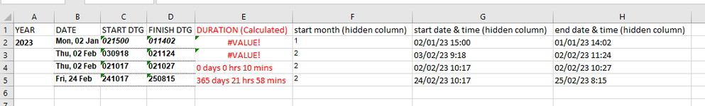
At work we use an uncommon format for the date and time of DDHHMM and month MMM (known as a DTG) It is standard in our area of work, but probable not much elsewhere and as Excel doesn’t know what a DTG is I use hidden formula to build it into something Excel will recognise.
My problem stems from calculating the days, hours and minutes between date/times, despite Excel recognising a “constructed” date and time i.e. dd/mm/yy hh:mm I cannot get the formula(s) I’ve tried to calculate correctly for every line of data;
As an example, it is okay with 02/02/23 10:17 to 02/02/23 10:27 It knows that is 10 minutes. However, it doesn’t like 02/02/23 09:18 to 05/02/23 08:00 which it seems to think is 1095 days, 22 hours and 42 minutes apart.
And it certainly doesn’t like calculating from 24/02/23 09:10 to 12/03/23 09:17
My system will not let me upload the spreadsheet as an example however I will include a screenshot, and what formula I am trying at the moment
Finally, much as I like Macro, I cannot use them in this project as work are paranoid about the vulnerability of coding (sadly).
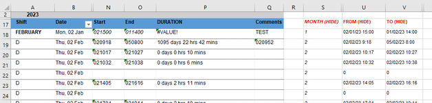
FORMULA BEING TRIED:
(column) P formula :
INT(V18-U18)&" days "&TEXT(V18-U18,"h"" hrs ""m"" mins """)
(column) S:
MONTH(B18)
(column) U:
TEXT((DATE($A$2,$S18,LEFT($N18,2))),"dd/mm/yy")&" "&TEXT((TIME(MID($N18,3,2),RIGHT($N18,2),0)),"h:mm")
(column) V:
IF(LEFT(O18,2)<LEFT(N18,2),TEXT((DATE($A$2,($S18+1),LEFT($O18,2))),"dd/mm/yy")&" "&TEXT((TIME(MID($O18,3,2),RIGHT($O18,2),0)),"h:mm"),TEXT((DATE($A$2,$S18,LEFT($O18,2))),"dd/mm/yy")&" "&TEXT((TIME(MID($O18,3,2),RIGHT($O18,2),0)),"h:mm"))
Thank you in anticipation!
It has been a long time since I’ve been here and/or done anything exciting with Excel, and I’ve forgotten quite a lot ☹ However I know you guys & gals are unmatchable, therefore: help please!
At work we use an uncommon format for the date and time of DDHHMM and month MMM (known as a DTG) It is standard in our area of work, but probable not much elsewhere and as Excel doesn’t know what a DTG is I use hidden formula to build it into something Excel will recognise.
My problem stems from calculating the days, hours and minutes between date/times, despite Excel recognising a “constructed” date and time i.e. dd/mm/yy hh:mm I cannot get the formula(s) I’ve tried to calculate correctly for every line of data;
As an example, it is okay with 02/02/23 10:17 to 02/02/23 10:27 It knows that is 10 minutes. However, it doesn’t like 02/02/23 09:18 to 05/02/23 08:00 which it seems to think is 1095 days, 22 hours and 42 minutes apart.
And it certainly doesn’t like calculating from 24/02/23 09:10 to 12/03/23 09:17
My system will not let me upload the spreadsheet as an example however I will include a screenshot, and what formula I am trying at the moment
Finally, much as I like Macro, I cannot use them in this project as work are paranoid about the vulnerability of coding (sadly).
FORMULA BEING TRIED:
(column) P formula :
INT(V18-U18)&" days "&TEXT(V18-U18,"h"" hrs ""m"" mins """)
(column) S:
MONTH(B18)
(column) U:
TEXT((DATE($A$2,$S18,LEFT($N18,2))),"dd/mm/yy")&" "&TEXT((TIME(MID($N18,3,2),RIGHT($N18,2),0)),"h:mm")
(column) V:
IF(LEFT(O18,2)<LEFT(N18,2),TEXT((DATE($A$2,($S18+1),LEFT($O18,2))),"dd/mm/yy")&" "&TEXT((TIME(MID($O18,3,2),RIGHT($O18,2),0)),"h:mm"),TEXT((DATE($A$2,$S18,LEFT($O18,2))),"dd/mm/yy")&" "&TEXT((TIME(MID($O18,3,2),RIGHT($O18,2),0)),"h:mm"))
Thank you in anticipation!