Hello All,
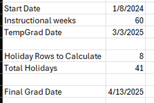
Looking for some support with this one. I will do my best to explain it. I am trying to dynamically calculate the end date of a program of study by using the start date and the number of program days (easy enough), while dynamically including/accounting for the established holidays that would fall within the length of that program.
So, for example, let's say the program starts on January 1st and is 20 days long, however, there is a holiday on 1/10 and day 1/19, so the end date really needs to be 22 days after the start date instead of 20.
Another example, a program that is 20 days long starts on 1/11 with the same holidays as above. For this entry, the calculation would return an end date based on 21 days because it starts after the holiday on 1/10.
The holiday dates are pre-established. Currently, I am attempting to have the holidays listed in one table and then have the program start date and number of days be what someone would enter to have the end date dynamically generated from referencing the list of holidays that would fall within the range of that program. And, I am lost bouncing between some VLOOKUP, INDEX, MATCH, and COUNTIFS. LOL
Any help would be appreciated.
Brad