reference on 4 conditions

Kenjiorson

New Member
Joined
Oct 25, 2023
Messages
15
Platform
  1. Windows
Hi i got a few add on need to seek help from the experts here again.

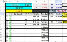
E5 - is reference, either 1, 2, S1 or S2.

H5 - i want to put in formula to add the time i manual key in G5. And read from E5 what i input, 1=60mins, 2=90mins, S1=45mins and S2=90mins
My current formula is - =$G6+TIME(0,IF($E6=1,60,IF($E6=2,90,IF($E6="S1",45,IF($E6="S2",120)))),0)
Also how to hide cell H9 to H14
I5 - Based on what i input in E5, 1=110, 2=150, S1=90 and S2=200.
My current formula - =if(E5=1,"110", if(E5=2,"150"))

J5 - Based on what i input in E5, 1=60 mins, 2=90 mins, S1=45 mins and S2=120 mins.
My current formula - =if(E5=1,"60 mins", if(E5=2,"90 mins"))

Thank you
 

Attachments

  • Sheet SS.jpg
    Sheet SS.jpg
    98.6 KB · Views: 7

Excel Facts

Get help while writing formula
Click the italics "fx" icon to the left of the formula bar to open the Functions Arguments dialog. Help is displayed for each argument.
Hello
I would like to look at it, but I need the file.
Your explanation is too confusing to me.
Or you can use this new add in to paste a mini-sheet in your message.
Regards,
EF
 
Upvote 0
Hello
I would like to look at it, but I need the file.
Your explanation is too confusing to me.
Or you can use this new add in to paste a mini-sheet in your message.
Regards,
EF
Hi i tried very long, no idea how to download. Tried for more than 30 minutes and it shows protected sheet
 
Last edited:
Upvote 0
H5: =IFERROR(VLOOKUP(E5,{1,60;2,90;"S1",45;"S2",90},2,0),0)& " mins"
I5: =IFERROR(VLOOKUP(E5,{1,110;2,150;"S1",90;"S2",200},2,0),0)
J5: =IFERROR(VLOOKUP(E5,{1,60;2,90;"S1",45;"S2",120},2,0),0)& " mins"
 
Upvote 0
H5: =IFERROR(VLOOKUP(E5,{1,60;2,90;"S1",45;"S2",90},2,0),0)& " mins"
I5: =IFERROR(VLOOKUP(E5,{1,110;2,150;"S1",90;"S2",200},2,0),0)
J5: =IFERROR(VLOOKUP(E5,{1,60;2,90;"S1",45;"S2",120},2,0),0)& " mins"
Hi thank you so much
H5 can help to edit the formula

Meaning:
I want the minutes auto add and show in H5 from what i input in E5 and G5.

Example:
G5 input 5pm and E5 input S1, H5 will show 5:45pm

Thank you
 
Upvote 0
H5: =$G6+(IFERROR(VLOOKUP(E5,{1,60;2,90;"S1",45;"S2",90},2,0),0)/1440)
J5: =$G6+(IFERROR(VLOOKUP(E5,{1,60;2,90;"S1",45;"S2",120},2,0),0)/1440)
 
Upvote 0
Solution

Forum statistics

Threads
1,215,103
Messages
6,123,103
Members
449,096
Latest member
provoking

We've detected that you are using an adblocker.

We have a great community of people providing Excel help here, but the hosting costs are enormous. You can help keep this site running by allowing ads on MrExcel.com.
Allow Ads at MrExcel

Which adblocker are you using?

Disable AdBlock

Follow these easy steps to disable AdBlock

1)Click on the icon in the browser’s toolbar.
2)Click on the icon in the browser’s toolbar.
2)Click on the "Pause on this site" option.
Go back

Disable AdBlock Plus

Follow these easy steps to disable AdBlock Plus

1)Click on the icon in the browser’s toolbar.
2)Click on the toggle to disable it for "mrexcel.com".
Go back

Disable uBlock Origin

Follow these easy steps to disable uBlock Origin

1)Click on the icon in the browser’s toolbar.
2)Click on the "Power" button.
3)Click on the "Refresh" button.
Go back

Disable uBlock

Follow these easy steps to disable uBlock

1)Click on the icon in the browser’s toolbar.
2)Click on the "Power" button.
3)Click on the "Refresh" button.
Go back
Back
Top