Relation column depends on condition (Power Pivot)

bukimi

Board Regular
Joined
Apr 12, 2017
Messages
105
Office Version
  1. 2019
Platform
  1. Windows
Hello,
I always solved problems with VBA. Recently, I had 4-day training in Power BI and I start solving more with it instead (easier on customer side).

I have two files that need to interact with each other. One is supposed to be gathering sum of sales value per customer. Second table is "raw data" with all sales listed. The problem is, that first table lists customers by ID that is divided accross several columns in sales data (second table). Maybe it's better to show on example data (attached).

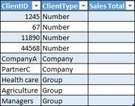
First table: Client ID (first column) is different by type. The type of ID is listed in second column (sorry, I can't install plugin to post in BB code, so I attach it as images)
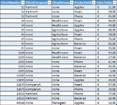
Second table: "Raw data" that has all sales of all customers. No column is unique, but client is identified by first 3 columns (number, company, group). Raw data is stored in separate file.

Relation between tables depends on "ClientType" in first table. It should sum values either by column A, or column B or column C in raw data (table2)... Don't know how to get around this obstacle.
I did solve counting with nested (many) IF and SUMIFS formula, but it's both very slow and complicated to refresh data on client side. It would be much easier, if I could just replace raw data file on server and make Power BI read from it and sum values accordingly.

A formula solution to example. Real, final formula for real data is much longer (more types, more conditions):
Excel Formula:
=IF([@ClientType]="Number",SUMIFS(Tabela2[Sales Value],Tabela2[ClientNumber],[@ClientID]),IF([@ClientType]="Company",SUMIFS(Tabela2[Sales Value],Tabela2[ClientCompany],[@ClientID]),IF([@ClientType]="Group",SUMIFS(Tabela2[Sales Value],Tabela2[ClientGroup],[@ClientID]),0)))

Any tips how to proceed with getting data in table 1 by setting relation to Table 2?
 

Attachments

  • exampleTable1.jpg
    exampleTable1.jpg
    23.2 KB · Views: 10
  • exampleTable2.jpg
    exampleTable2.jpg
    101.7 KB · Views: 10

Excel Facts

Do you hate GETPIVOTDATA?
Prevent GETPIVOTDATA. Select inside a PivotTable. In the Analyze tab of the ribbon, open the dropown next to Options and turn it off
For a Relationship to exist between two tables, one of them must have a column of unique values that the other table uses for one or more rows.
Your two tables are completely inconsistent. The table with ClientID had values used in two different columns in table with ClientNumber.
What you're looking to do is easy enough to do with a formula once the data makes sense.
Book1
ABCD
26ClientNumberClientCompanyClientGroupSalesTotal
2712PartnerCnone$ 115.00
2834noneHealth care$ 138.00
2945noneAgriculture$ 305.00
3067nonenone$ 55.00
311109noneHealth care$ 114.00
321245nonenone$ 131.00
331279CompanyAnone$ 127.00
3411200nonenone$ 14.00
3511890nonenone$ 49.00
3614550PartnerCnone$ 101.00
3744568noneManagers$ 32.00
Sheet2
Cell Formulas
RangeFormula
D27:D37D27=SUMIFS(fRawData[SalesValue],fRawData[ClientNumber],[@ClientNumber])

Alternately, you could pull the two corrected tables into Power Query and get the same result merging the tables:
Power Query:
let
    Source = Excel.CurrentWorkbook(){[Name="dCustSalesPQ"]}[Content],
    ChangedType = Table.TransformColumnTypes(Source,{{"ClientNumber", Int64.Type}, {"ClientCompany", type text}, {"ClientGroup", type text}}),
    MergedQueries = Table.NestedJoin(ChangedType, {"ClientNumber"}, fRawData, {"ClientNumber"}, "fRawData", JoinKind.LeftOuter),
    AggregatedfRawData = Table.AggregateTableColumn(MergedQueries, "fRawData", {{"SalesValue", List.Sum, "Sum of SalesValue"}}),
    ChangedType1 = Table.TransformColumnTypes(AggregatedfRawData,{{"Sum of SalesValue", Int64.Type}})
in
    ChangedType1
But first you have to clean up the data! Also, PLEASE use XL2BB to post data samples. It takes FOREVER to transcribe pictures!
 
Upvote 0
Sorry about the pictures. I had no way to install any add-in to my Excel on company computer. I also had to make example data.
Thank you for your help. I have no influence on the way that input (raw data) or output data (small Table1) look like, because I'm receiving input from server and transform it to a very specific needs for someone else... I know it's messy and inconsistent, that's why I needed help in the first place ;)

I need SalesTotal calculated in the first messy table, not the second one. I mean, it has to remain "messy" with ClientID being either a number, or a type - determined by description in another column. Even if I make ClientNumber a unique column in raw data (add products values together), it's still pairing only with "Number" client type in first table, when I put a relation between tables.
It's like tables should be related by ClientNumber: when messy table asks for total of a number and related by Group: when messy table asks for total of a group (which consists of several client numbers). That's not easy and not something they teach on Power BI courses (sadly).

I also rewrote the same data onto another computer, to make it in XL2BB. I attach it now.
Zeszyt1
ABC
1ClientIDClientTypeSalesTotal
21245Number
367Number
411980Number
544568Number
6CompanyACompany
7PartnerCCompany
8Health careGroup
9AgricultureGroup
10ManagersGroup
Arkusz1


Zeszyt1
EFGHI
1ClientNumberClientCompanyClientGroupProductSold Sales Value
212PartnerCnoneApples€ 11,00
312PartnerCnonePears€ 19,00
412PartnerCnonePlums€ 85,00
534noneHealth carePears€ 94,00
634noneHealth careApples€ 44,00
745noneAgricultureApples€ 88,00
845noneAgriculturePears€ 59,00
945noneAgriculturePlums€ 75,00
1045noneAgricultureBananas€ 83,00
1167noneAgriculturePears€ 55,00
121109nonenonePears€ 97,00
131109noneHealth careBananas€ 17,00
141245noneHealth carePlums€ 81,00
151245nonenoneBananas€ 45,00
161245nonenonePears€ 5,00
1711200nonenoneBananas€ 14,00
1811890nonenoneApples€ 49,00
1912679CompanyAnonePears€ 97,00
2012679CompanyAnonePlums€ 30,00
2114550PartnerCnonePlums€ 77,00
2214550PartnerCnoneBananas€ 24,00
2344568noneManagersApples€ 32,00
Arkusz1
 
Upvote 0
I turned the second set of data into a Table named Sales, I found it harder to work with the output as a Table which I hardly ever do. I came up with this:
Book1
ABC
1ClientIDClientTypeSalesTotal
21245Number131
367Number55
411980NumberNOT FOUND
544568Number32
6CompanyACompany127
7PartnerCCompany216
8Health careGroup236
9AgricultureGroup360
10ManagersGroup32
Sheet1
Cell Formulas
RangeFormula
C2:C10C2=IFS( NOT(ISERROR(MATCH(A2,Sales[ClientNumber],0))), SUMIFS(Sales[Sales Value],Sales[ClientNumber],A2), NOT(ISERROR(MATCH(A2,Sales[ClientCompany],0))), SUMIFS(Sales[Sales Value],Sales[ClientCompany],A2), NOT(ISERROR(MATCH(A2,Sales[ClientGroup],0))), SUMIFS(Sales[Sales Value],Sales[ClientGroup],A2), TRUE,"NOT FOUND")

I looked up functions to make sure it would work with 2019, so that should be good. Of note, the ISERR function didn't work and had to use IFERROR instead. Go figure! I broke up the formula with returns to help make the formula a bit clearer. And no, that doesn't use the Client Type column because using it wasn't showing when the ClientID wasn't found. It is a simpler formula though:
Excel Formula:
=IFS(
B2="Number", SUMIFS(Sales[Sales Value],Sales[ClientNumber],A2),
B2="Company", SUMIFS(Sales[Sales Value],Sales[ClientCompany],A2),
B2="Group",      SUMIFS(Sales[Sales Value],Sales[ClientGroup],A2),
TRUE,"NOT FOUND")
I left the TRUE statement in just in case there's no match for any of the three groups.
I've been there too, and sometimes you have to work with the junk you're given, but that's really a mess!
Hope that helps, and good luck!
 
Upvote 0
Thank you.
I got the formula part before. I actually posted a similar one in my first post. The problem with using formulas is that Excel works slowly when there are many of them - any changes to "messy table" makes it recalculate everything. It's also harder to manage when conditions change. Switching to manual calculation helps only a little. That's why I preferred Power Query solution, so refreshing pulls new data and recalculates it - it's easier to replace raw data with new data, too. (simple replacing source file in a folder does the trick)

I figured out something to try, sitting and thinking about it. I'll try it in on Monday.
1. Add both data sets by Power Query (they are usually separate files).
2. Transform raw data with Power Query, a few times, making different final table everytime:
Firstly, group sales by client number - it would finally have two columns only: client number and sales total. Let's call it "NumberTable".
Then, group sales by company - it would finally have two columns, too. Let's call it "CompanyTable".
3. Proceed similarly with all client types. Finally, join all tables together, one below another, making one big data table, where first column is unique key (it's either a number, a company, or a group). Of course making any "total sum" directly out of it would be a bad idea, since sales values may and will be duplicated among different keys.
4. First "messy table" then gets related one-to-one to joined data, pulling values by unique key. It doesn't even need to check contents of second column.
 
Upvote 0
Then lets try Power Query. This is NOT efficient to set up, and I'm sure there are others that could do this a LOT more elegantly, but this does get the job done. I start with this:
Book1
ABCDEFGH
1BlankReportSales
2ClientIDClientTypeClientNumberClientCompanyClientGroupProductSold Sales Value
31245Number12PartnerCnoneApples11
467Number12PartnerCnonePears19
511980Number12PartnerCnonePlums85
644568Number34noneHealth carePears94
7CompanyACompany34noneHealth careApples44
8PartnerCCompany45noneAgricultureApples88
9Health careGroup45noneAgriculturePears59
10AgricultureGroup45noneAgriculturePlums75
11ManagersGroup45noneAgricultureBananas83
1267noneAgriculturePears55
131109nonenonePears97
141109noneHealth careBananas17
151245noneHealth carePlums81
161245nonenoneBananas45
171245nonenonePears5
1811200nonenoneBananas14
1911890nonenoneApples49
2012679CompanyAnonePears97
2112679CompanyAnonePlums30
2214550PartnerCnonePlums77
2314550PartnerCnoneBananas24
2444568noneManagersApples32
Sheet1

The names in Row 1 are the table names.
Step 1 is to pull in the Sales report table,
Power Query:
let
    Source = Excel.CurrentWorkbook(){[Name="Sales"]}[Content],
    ChangedType = Table.TransformColumnTypes(Source,{{"ClientNumber", Int64.Type}, {"ClientCompany", type text}, {"ClientGroup", type text}, {"ProductSold", type text}, {" Sales Value ", Int64.Type}})
in
    ChangedType
and then Reference it to three other reports named Number, Company, and Group. Each of those copies groups by the column indicated by its name to get the total sales for each of the items in that column.
Number is transformed like this:
Power Query:
let
    Source = Sales,
    GroupedRows = Table.Group(Source, {"ClientNumber"}, {{"Sales", each List.Sum([#" Sales Value "]), type nullable number}})
in
    GroupedRows
Company like this:
Power Query:
let
    Source = Sales,
    GroupedRows = Table.Group(Source, {"ClientCompany"}, {{"Sales", each List.Sum([#" Sales Value "]), type nullable number}})
in
    GroupedRows
and Group like this:
Power Query:
let
    Source = Sales,
    GroupedRows = Table.Group(Source, {"ClientGroup"}, {{"Sales", each List.Sum([#" Sales Value "]), type nullable number}})
in
    GroupedRows
These tables are the result, but I show them just for clarity:
Book1
NOPQRSTU
1NumberCompanyGroup
2ClientNumberSalesClientCompanySalesClientGroupSales
312115PartnerC216none553
434138none838Health care236
545305CompanyA127Agriculture360
66755Managers32
71109114
81245131
91120014
101189049
1112679127
1214550101
134456832
Sheet1

They can be loaded as a Connection Only. Now those three tables are merged with the blank report from above like this:
Power Query:
let
    Source = Excel.CurrentWorkbook(){[Name="BlankReport"]}[Content],
    MergedClientID = Table.NestedJoin(Source, {"ClientID"}, Number, {"ClientNumber"}, "Number", JoinKind.LeftOuter),
    ExpandedClientIdSales = Table.ExpandTableColumn(MergedClientID, "Number", {"Sales"}, {"ID Sales"}),
    MergedCompany = Table.NestedJoin(ExpandedClientIdSales, {"ClientID"}, Company, {"ClientCompany"}, "Company", JoinKind.LeftOuter),
    ExpandedCompanySales = Table.ExpandTableColumn(MergedCompany, "Company", {"Sales"}, {"Company Sales"}),
    MergedGroup = Table.NestedJoin(ExpandedCompanySales, {"ClientID"}, Group, {"ClientGroup"}, "Group", JoinKind.LeftOuter),
    ExpandedGroup = Table.ExpandTableColumn(MergedGroup, "Group", {"Sales"}, {"Group Sales"}),
    MergedSales = Table.CombineColumns(Table.TransformColumnTypes(ExpandedGroup, {{"ID Sales", type text}, {"Company Sales", type text}, {"Group Sales", type text}}, "en-US"),{"ID Sales", "Company Sales", "Group Sales"},Combiner.CombineTextByDelimiter("", QuoteStyle.None),"Total Sales"),
    ChangedType = Table.TransformColumnTypes(MergedSales,{{"ClientID", type any}, {"ClientType", type text}, {"Total Sales", Int64.Type}})
in
    ChangedType
Which produces this report:
Book1
JKL
1SalesReport
2ClientIDClientTypeTotal Sales
31245Number131
467Number55
544568Number32
611980Number
7CompanyACompany127
8PartnerCCompany216
9Health careGroup236
10AgricultureGroup360
11ManagersGroup32
Sheet1

It's worth noting that if the Sales table is updated, the Sales Report is updated by just going to the Data tab and selecting Refresh All. If the Sales data is coming in from an external source, it can be imported and the report updated by that same click.
Power Query is VERY powerful and worth learning. Hope that works for you.
 
Upvote 0
Another way:

Power Query:
let
    Rpt = Excel.CurrentWorkbook(){[Name="ReportTemplate"]}[Content],
    Sales = Excel.CurrentWorkbook(){[Name="Sales"]}[Content],
    tbl = Table.AddColumn(Rpt, "SalesTotal", each 
            List.Sum(Table.SelectRows(Sales, (x)=> Record.Field(x, "Client" & [ClientType]) = [ClientID])[Sales Value]))
in
    tbl

Book1
ABCDEFGHIJKLM
1ReportTemplateSalesQuery Output
2
3ClientIDClientTypeClientNumberClientCompanyClientGroupProductSoldSales ValueClientIDClientTypeSalesTotal
41245Number12PartnerCnoneApples111245Number131
567Number12PartnerCnonePears1967Number55
611890Number12PartnerCnonePlums8511890Number49
744568Number34noneHealth carePears9444568Number32
8CompanyACompany34noneHealth careApples44CompanyACompany127
9PartnerCCompany45noneAgricultureApples88PartnerCCompany216
10Health careGroup45noneAgriculturePears59Health careGroup236
11AgricultureGroup45noneAgriculturePlums75AgricultureGroup360
12ManagersGroup45noneAgricultureBananas83ManagersGroup32
1367noneAgriculturePears55
141109nonenonePears97
151109noneHealth careBananas17
161245noneHealth carePlums81
171245nonenoneBananas45
181245nonenonePears5
1911200nonenoneBananas14
2011890nonenoneApples49
2112679CompanyAnonePears97
2212679CompanyAnonePlums30
2314550PartnerCnonePlums77
2414550PartnerCnoneBananas24
2544568noneManagersApples32
26
Sheet2
 
Upvote 0
Another way:

Power Query:
let
    Rpt = Excel.CurrentWorkbook(){[Name="ReportTemplate"]}[Content],
    Sales = Excel.CurrentWorkbook(){[Name="Sales"]}[Content],
    tbl = Table.AddColumn(Rpt, "SalesTotal", each
            List.Sum(Table.SelectRows(Sales, (x)=> Record.Field(x, "Client" & [ClientType]) = [ClientID])[Sales Value]))
in
    tbl

Book1
ABCDEFGHIJKLM
1ReportTemplateSalesQuery Output
2
3ClientIDClientTypeClientNumberClientCompanyClientGroupProductSoldSales ValueClientIDClientTypeSalesTotal
41245Number12PartnerCnoneApples111245Number131
567Number12PartnerCnonePears1967Number55
611890Number12PartnerCnonePlums8511890Number49
744568Number34noneHealth carePears9444568Number32
8CompanyACompany34noneHealth careApples44CompanyACompany127
9PartnerCCompany45noneAgricultureApples88PartnerCCompany216
10Health careGroup45noneAgriculturePears59Health careGroup236
11AgricultureGroup45noneAgriculturePlums75AgricultureGroup360
12ManagersGroup45noneAgricultureBananas83ManagersGroup32
1367noneAgriculturePears55
141109nonenonePears97
151109noneHealth careBananas17
161245noneHealth carePlums81
171245nonenoneBananas45
181245nonenonePears5
1911200nonenoneBananas14
2011890nonenoneApples49
2112679CompanyAnonePears97
2212679CompanyAnonePlums30
2314550PartnerCnonePlums77
2414550PartnerCnoneBananas24
2544568noneManagersApples32
26
Sheet2
KNEW there was a MUCH better way! Very cool.
 
Upvote 0

Forum statistics

Threads
1,215,469
Messages
6,124,989
Members
449,201
Latest member
Lunzwe73

We've detected that you are using an adblocker.

We have a great community of people providing Excel help here, but the hosting costs are enormous. You can help keep this site running by allowing ads on MrExcel.com.
Allow Ads at MrExcel

Which adblocker are you using?

Disable AdBlock

Follow these easy steps to disable AdBlock

1)Click on the icon in the browser’s toolbar.
2)Click on the icon in the browser’s toolbar.
2)Click on the "Pause on this site" option.
Go back

Disable AdBlock Plus

Follow these easy steps to disable AdBlock Plus

1)Click on the icon in the browser’s toolbar.
2)Click on the toggle to disable it for "mrexcel.com".
Go back

Disable uBlock Origin

Follow these easy steps to disable uBlock Origin

1)Click on the icon in the browser’s toolbar.
2)Click on the "Power" button.
3)Click on the "Refresh" button.
Go back

Disable uBlock

Follow these easy steps to disable uBlock

1)Click on the icon in the browser’s toolbar.
2)Click on the "Power" button.
3)Click on the "Refresh" button.
Go back
Back
Top