Return Vertical number header based horizontal number header and number into a matrix

marreco

Well-known Member
Joined
Jan 1, 2011
Messages
609
Office Version
  1. 2010
Platform
  1. Windows
I have a table start in A1 goes G31, [B2:G2] is number header as columns and in [A2:31 number that a need return], my search matrix is in [B3:G31].
How return intersection values?

X
4,2​
5​
6,3​
8​
10​
12,5​
5​
2,77​
4​
6,3​
10​
16​
25​
5,5​
2,52​
3,64​
5,73​
9,09​
14,55​
22,73​
6​
2,31​
3,33​
5,25​
8,33​
13,33​
20,83​
6,5​
2,13​
3,08​
4,85​
7,69​
12,31​
19,23​
7​
1,98​
2,86​
4,5​
7,14​
11,43​
17,86​
7,5​
1,85​
2,67​
4,2​
6,67​
10,67​
16,67​
8​
1,73​
2,5​
3,94​
6,25​
10​
15,63​
8,5​
1,63​
2,35​
3,71​
5,88​
9,41​
14,71​
9​
1,54​
2,22​
3,5​
5,56​
8,89​
13,89​
9,5​
1,46​
2,11​
3,32​
5,26​
8,42​
13,16​
10​
1,39​
2​
3,15​
5​
8​
12,5​
11​
1,26​
1,82​
2,86​
4,55​
7,27​
11,36​
12​
1,15​
1,67​
2,62​
4,17​
6,67​
10,42​
12,5​
1,11​
1,6​
2,52​
4​
6,4​
10​
13​
1,07​
1,54​
2,42​
3,85​
6,15​
9,62​
14​
0,99​
1,43​
2,25​
3,57​
5,71​
8,93​
15​
0,92​
1,33​
2,1​
3,33​
5,33​
8,33​
16​
0,87​
1,25​
1,97​
3,13​
5​
7,81​
17​
0,81​
1,18​
1,85​
2,94​
4,71​
7,35​
17,5​
0,79​
1,14​
1,8​
2,86​
4,57​
7,14​
18​
0,77​
1,11​
1,75​
2,78​
4,44​
6,94​
19​
0,73​
1,05​
1,66​
2,63​
4,21​
6,58​
20​
0,69​
1​
1,58​
2,5​
4​
6,25​
22​
0,63​
0,91​
1,43​
2,27​
3,64​
5,68​
24​
0,58​
0,83​
1,31​
2,08​
3,33​
5,21​
25​
0,55​
0,8​
1,26​
2​
3,2​
5​
26​
0,53​
0,77​
1,21​
1,92​
3,08​
4,81​
28​
0,49​
0,71​
1,12​
1,79​
2,86​
4,46​
30​
0,46​
0,67​
1,05​
1,67​
2,67​
4,17​
33​
0,42​
0,61​
0,95​
1,52​
2,42​
3,79​
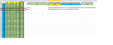
Lookup this value(exact or greater than)Find this vertical HeaderReturn this from horizontal headerReturn this from Matrix
1912,56,519,23
Cell K2=DESLOC(ÍNDICE(B2:G31;How_find_row_here;CORRESP(J2;B1:G1;0));0;-CORRESP(J2;B1:G1;0))
Cell L2=ÍNDICE(B2:G31;How_find_row_here;CORRESP(J2;B1:G1;0))
 

Attachments

  • look_at_me.png
    look_at_me.png
    45.6 KB · Views: 6
Last edited by a moderator:

Excel Facts

Round to nearest half hour?
Use =MROUND(A2,"0:30") to round to nearest half hour. Use =CEILING(A2,"0:30") to round to next half hour.
I suggest that you update your Account details (or click your user name at the top right of the forum) so helpers always know what Excel version(s) & platform(s) you are using as the best solution often varies by version. (Don’t forget to scroll down & ‘Save’)

How about
+Fluff 1.xlsm
ABCDEFGHIJKL
1X4.256.381012.5
252.7746.31016251912.56.519.23
35.52.523.645.739.0914.5522.73
462.313.335.258.3313.3320.83
56.52.133.084.857.6912.3119.23
671.982.864.57.1411.4317.86
77.51.852.674.26.6710.6716.67
881.732.53.946.251015.63
98.51.632.353.715.889.4114.71
1091.542.223.55.568.8913.89
119.51.462.113.325.268.4213.16
12101.3923.155812.5
13111.261.822.864.557.2711.36
14121.151.672.624.176.6710.42
1512.51.111.62.5246.410
16131.071.542.423.856.159.62
17140.991.432.253.575.718.93
18150.921.332.13.335.338.33
19160.871.251.973.1357.81
20170.811.181.852.944.717.35
2117.50.791.141.82.864.577.14
22180.771.111.752.784.446.94
23190.731.051.662.634.216.58
24200.6911.582.546.25
25220.630.911.432.273.645.68
26240.580.831.312.083.335.21
27250.550.81.2623.25
28260.530.771.211.923.084.81
29280.490.711.121.792.864.46
30300.460.671.051.672.674.17
31330.420.610.951.522.423.79
Lists
Cell Formulas
RangeFormula
L2L2=INDEX(B2:G31,MATCH(K2,A2:A31,0),MATCH(J2,B1:G1,0))
 
Upvote 0
Hi Fluff, I already try this before open this post here, but din't work.
If put in I2=4 and J2=8, then result would be K2=12,5 and L2=4
If put in I2=3 and J2=8, then result would be K2=16 and L2=3,13 (3 is not in table then get close up number there)
 
Upvote 0
Ok, for K2 use
Excel Formula:
=INDEX(A2:A31,MATCH(I2,INDEX(B2:G31,,MATCH(J2,B1:G1,0)),-1))
 
Upvote 0

Forum statistics

Threads
1,215,137
Messages
6,123,253
Members
449,093
Latest member
Vincent Khandagale

We've detected that you are using an adblocker.

We have a great community of people providing Excel help here, but the hosting costs are enormous. You can help keep this site running by allowing ads on MrExcel.com.
Allow Ads at MrExcel

Which adblocker are you using?

Disable AdBlock

Follow these easy steps to disable AdBlock

1)Click on the icon in the browser’s toolbar.
2)Click on the icon in the browser’s toolbar.
2)Click on the "Pause on this site" option.
Go back

Disable AdBlock Plus

Follow these easy steps to disable AdBlock Plus

1)Click on the icon in the browser’s toolbar.
2)Click on the toggle to disable it for "mrexcel.com".
Go back

Disable uBlock Origin

Follow these easy steps to disable uBlock Origin

1)Click on the icon in the browser’s toolbar.
2)Click on the "Power" button.
3)Click on the "Refresh" button.
Go back

Disable uBlock

Follow these easy steps to disable uBlock

1)Click on the icon in the browser’s toolbar.
2)Click on the "Power" button.
3)Click on the "Refresh" button.
Go back
Back
Top