Row to column like in the output

[Arunchira]

Row1 2 6 7
Row 2 20 5 8
Row 3 10
Row 4 45 46
Do you know the name of this Converon
Row 1 2
6
7
Row2. 20
5
8
Row3. 10
Row4. 45
46

 

[jolivanes]

Change references as and where required.

Sub Maybe()
Dim i As Long, sh2 As Worksheet, lc As Long
Set sh2 = Worksheets("Sheet2")
    For i = 2 To Cells(Rows.Count, 1).End(xlUp).Row
        lc = Cells(i, Columns.Count).End(xlToLeft).Column
            sh2.Cells(Rows.Count, 2).End(xlUp).Offset(1, -1).Resize(, 2).Value = Cells(i, 1).Resize(, 2).Value
        If lc > 2 Then sh2.Cells(Rows.Count, 2).End(xlUp).Offset(1).Resize(lc - 2).Value = Application.Transpose(Cells(i, 3).Resize(, lc - 2).Value)
    Next i
End Sub

 

[Anonymous1378]

Try this?

=LET(
_a,A1:D3,
_b,TOCOL(EXPAND(TAKE(_a,,1),,COLUMNS(_a)-1,"")),
_c,TOCOL(DROP(_a,,1)&""),
FILTER(HSTACK(_b,_c),_c<>""))

 

[jolivanes]

Similar as Post #2 but different.
Change references as and where required.

Sub Maybe()
Dim i As Long, sh2 As Worksheet
Set sh2 = Worksheets("Sheet2")
    For i = 2 To Cells(Rows.Count, 1).End(xlUp).Row
        With sh2.Cells(Rows.Count, 2).End(xlUp).Offset(1)
            .Offset(, -1).Value = Cells(i, 1).Value
            .Resize(Cells(i, Columns.Count).End(xlToLeft).Column - 1).Value = _
            Application.Transpose(Cells(i, 1).Offset(, 1).Resize(, Cells(i, Columns.Count).End(xlToLeft).Column - 1).Value)
        End With
    Next i
End Sub

 

[Peter_SSs]

Welcome to the MrExcel board!

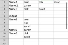
Assuming rows are filled from the left and each row has a value in column B at least, like your sample data, then another formula option to consider might be ...

23 08 26.xlsm
	A	B	C	D
1	Name1	arun	rob	sarah
2	Name2	danny
3	Name3	nick	david
4
5
6	Name1	arun
7		rob
8		sarah
9	Name2	danny
10	Name3	nick
11		david
12
Arunchira

Cell Formulas
Range	Formula
A6:B11	A6	=HSTACK(TOCOL(IF(COLUMN(B1:D3)>COLUMN(B1),IF(B1:D3="",x,""),A1:A3),2),TOCOL(B1:D3,1))
Dynamic array formulas.

 

[alansidman]

One more alternative is with Power Query to unpivot your data

Import your data to PQ editor (Get and Transform Data and found on the Data Tab of the ribbon)
Select first column and then on the Transform Tab, select Unpivot --> Unpivot other columns
On the Home tab, select Close and Load. Select your location.

let
    Source = Excel.CurrentWorkbook(){[Name="Table2"]}[Content],
    #"Unpivoted Other Columns" = Table.UnpivotOtherColumns(Source, {"Column1"}, "Attribute", "Value"),
    #"Removed Columns" = Table.RemoveColumns(#"Unpivoted Other Columns",{"Attribute"})
in
    #"Removed Columns"