After looking at the results while trying to write up an explanation, my formula does not work properly. Amazingly, it only works based on the order of your sample data. If you re-arrange the values in column A, it stops working.
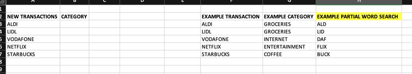
ALDI and LIDL return GROCERIES because the LOOKUP function is returning a 1 - but that '1' is from the position of the partial match in the string, not the position of the array returned by the SEARCH function. "ALD" and "LID" are found starting in position 1 of "ALDI" and "LIDL", respectively.
Same applies to VODAFONE ("OFA" is found in position 3, hence the third value, INTERNET, is returned. For NETFLIX, "FLIX" is in position 4 and for STARBUCKS, "BUCKS" is in position 5. So in each example it "successfully" match the correct row. Now I've seen it all, haha.
So some work still needs to be done with this one, but back to your original question about 9E+307...
9E+307 is a very, very large number (exponential notation, equivalent to 9 followed by 307 zeros) - greater than any number anyone is likely to enter into a cell. If LOOKUP doesn't find an exact match to that number it will return the next largest number it finds in the range/array. See the Excel help files for its usage, limitations and more details about how the function works.