Search a value across a range of two columns and return the first 10 results

[Abdmujib]

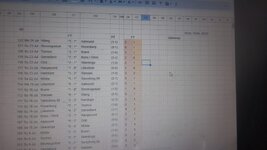
Hello, I have been trying find the value on DC4 that is (valenranga) from range of two columns i.e CS or CU for the first 10. It can either find it in either of the two colum the it should return corresponding result of CS, CT and CU.

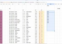
E.g the first and second results would be

Odd *2 - 1* Valenranga
Valenranga *0 - 4* Molde

For the three corresponding column respectively.


Pls Kindly don't mind the interface of google sheet i snapped

 

[Abdmujib]

For the first image named excel, I changed the DC6 in the IF condition to DA1, as you can see it only populate for the the first column from DA5.
For the 2nd image named ex2, I change the entire reference to other cell range to DG6:Dj18, and the llookup value to DH4. where as it suppose to search for it in DG6:DG18. it gives the result in DR.

I'm using the formula on google sheets, not Excel but the initial one works perfectly.

I will try your latest answer to see if it work and I will give you the feed back soon

thank you.
.

 

[Abdmujib]

If the value to search is in DC4, your list starts on CS5, and the output need to be created from DC5:DE5 then the formula should be entered using the CSE procedure in DC5:DE5 and should be

=IFERROR(INDEX($CS$1:$CU$998,SMALL(IF($CS$5:$CS$998=$DC$4,ROW($CS$5:$CS$998),""),ROW(A1)),{1,2,3}),"")

(with the doubt about the field separator within the braces {})

Gives the same answer with the previous one.

Don't worry sir. maybe I will use if and query function to achieve that. though it will only take more cells spaces to arrieved at the answer.

Thank you sir.

 

[Anthony47]

In GoogleSheets probably it is not necessary to enter the formula in all the three horizontal cells, nor using Contr-Shift-Enter: you set the formula in the first cell and hit Enter, and the result will spill to the two adjacent cells (as with Dynamic Arrays in Excel). Then you copy the formula down.
Keep in mind that in =IFERROR(INDEX(ArrayAddress,etc etc ArrayAddress must always start from row1; so it's wrong using for example INDEX($DG$6 that I see in your second image.

 

[Abdmujib]

In GoogleSheets probably it is not necessary to enter the formula in all the three horizontal cells, nor using Contr-Shift-Enter: you set the formula in the first cell and hit Enter, and the result will spill to the two adjacent cells (as with Dynamic Arrays in Excel). Then you copy the formula down.
Keep in mind that in =IFERROR(INDEX(ArrayAddress,etc etc ArrayAddress must always start from row1; so it's wrong using for example INDEX($DG$6 that I see in your second image.

Oh thank you for the enlightenment. yeah, the first question spilled into the other cells but didn't realised it was because it is google sheet.

Thank you once again